Neutral temperature and atmospheric water vapour retrieval from spectral fitting of auroral and airglow emissions

We have developed a spectral fitting method to retrieve upper atmospheric parameters at multiple altitudes simultaneously during times of aurora, allowing us to measure neutral temperatures and column densities of water vapour. We use the method to separate airglow OH emissions from auroral O⁺ and N₂ in observations between 725 and 740 nm using the High Throughput Imaging Echelle Spectrograph (HiTIES) located on Svalbard. In this paper, we describe our new method and show the results of Monte Carlo simulations using synthetic spectra which demonstrate the validity of the spectral fitting method and provide an indication of uncertainties on the retrieval of each atmospheric parameter. We show that the method allows for the retrieval of OH temperatures with an uncertainty of 6 % when contamination by N₂ emission is small. N₂ temperatures can be retrieved with uncertainties down to 3 %–5 % when N₂ emission intensity is high. We can determine the intensity ratio between the O⁺ doublets at 732 and 733 nm (which is a function of temperature) with an uncertainty of 5 %.

1 Introduction

Spectral observations are an important diagnostic tool to probe the upper atmosphere, a region that is difficult to measure directly. Emissions from this region include optical airglow and aurorae, which are produced by the de-excitation of atoms or molecules in the upper mesosphere and the thermosphere. These emissions contain information on the state of the layers of atmosphere in which they are produced and also on the solar photons or precipitating energetic particles responsible for the excited states of the atmospheric species. Furthermore, since optical emissions from the upper atmosphere are produced over a wide range of altitudes, by simultaneously observing at different wavelengths, it is possible to build up a picture of the vertical structure of the upper atmosphere.

The neutral temperature is one parameter that is possible to determine from spectral observations in visible wavelengths. Making the assumption that the emitting species are in local thermodynamic equilibrium (LTE), the neutral temperature can be obtained by measuring emissions from the rotational bands of molecules. In this way, neutral temperatures have been determined from observations of airglow emissions from the OH layer located near the mesopause (Chadney et al., 2017; French et al., 2000; Holmen et al., 2014; Phillips et al., 2004; Suzuki et al., 2010). It has also been possible to measure rotational temperatures from N${}_{\mathrm{2}}^{+}$ ions observed during aurorae (Jokiaho et al., 2008; Koehler et al., 1981).

One difficulty with these measurements is that emissions from different species often occur at the same wavelengths. For example, past studies of OH temperatures (such as those listed above) have not been able to obtain measurements during periods of auroral activity, when auroral emissions contaminate the OH spectrum. To overcome this problem, we have developed a method to distinguish different emissions seen in the High Throughput Imaging Echelle Spectrograph, HiTIES (Chakrabarti et al., 2001), by fitting the spectrum, thus enabling us to measure temperatures at different altitudes simultaneously.

Our spectral fitting method also allows for the determination of the column density of water vapour, or precipitable water vapour (PWV), by measuring the absorption of upper atmospheric airglow emissions. There are multiple other methods traditionally used to measure PWV, either from the ground using the Global Navigation Satellite System (GNSS) (Bevis et al., 1992; Yao et al., 2017), from radiosondes (Maturilli and Kayser, 2016), or from satellite observations (Chaboureau et al., 1998; Noël et al., 1999; Schluessel and Emery, 1990). However, polar regions pose certain difficulties for these methods. Indeed, there is a lack of stations for ground-based measurements, and satellite retrieval methods using microwave imagers require knowledge of the surface emissivity, which is large and highly variable over ice and snow (Melsheimer and Heygster, 2008). The optical ground-based measurement of PWV from airglow, described in this paper, allows for estimates of atmospheric water vapour column densities at high temporal resolution in the Arctic.

The instrument is described in Sect. 2, and the different emissions it measures are described in Sect. 3. Section 4 details the spectral fitting and temperature retrieval process. We have run a Monte Carlo simulation to quantify the uncertainties on parameter retrieval from the HiTIES spectra; the results of these retrieval tests are discussed in Sect. 5. Monte Carlo simulations also allow us to assess uncertainties on the laboratory measurements of quantum numbers required to determine OH temperatures, as described in Sect. 6.

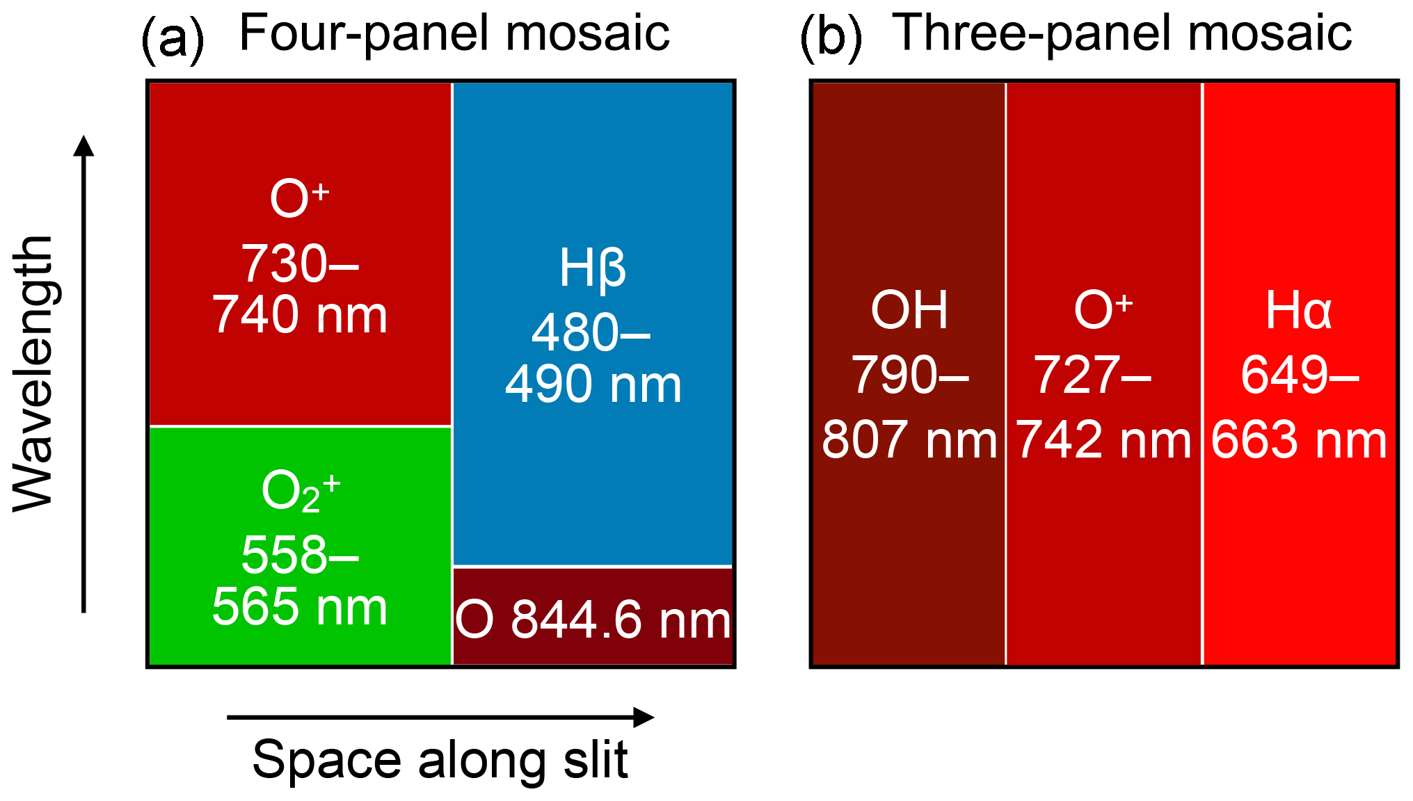
Figure 1 Diagrams showing the different wavebands of some mosaic interference filters used with HiTIES. The four-panel mosaic (a) has been in use for most seasons between 2003 and 2015; the three-panel mosaic (b) has been in use since December 2015.

2 HiTIES

The High Throughput Imaging Echelle Spectrograph (Chakrabarti et al., 2001) has been measuring emissions from the upper polar atmosphere since the year 2000. It is a part of the Spectrographic Imaging Facility (SIF) located in the high Arctic on Svalbard at the Kjell Henriksen Observatory (78.148^∘ N, 16.043^∘ E). The spectrograph has an 8^∘ slit that is centred on the magnetic zenith. Light entering the instrument passes through a collimator, before being diffracted by an echelle grating and re-imaged on an EMCCD detector. A mosaic of interference filters is used to separate overlapping diffraction orders, allowing for the simultaneous observation at high temporal and spectral resolution of non-contiguous spectral regions. Figure 1 shows a schematic diagram of the two mosaic filters that have been used the most often over the lifetime of the instrument. Each individual panel of the filters is centred in wavelength on a particular atmospheric emission of interest, although it should be noted that each panel may also contain emissions from multiple other species.

The instrument records images at a frequency of 2 Hz; however, depending on the brightness of the observed emissions, the spectra are typically post-integrated to between ∼10 and 120 s. The width of the spectrograph slit can be changed to adjust the spectral resolution, with higher resolution being a trade-off with the amount of light captured. In the 2015–2016 season, during which the data in Fig. 2 were recorded, the FWHM was 0.15 nm.

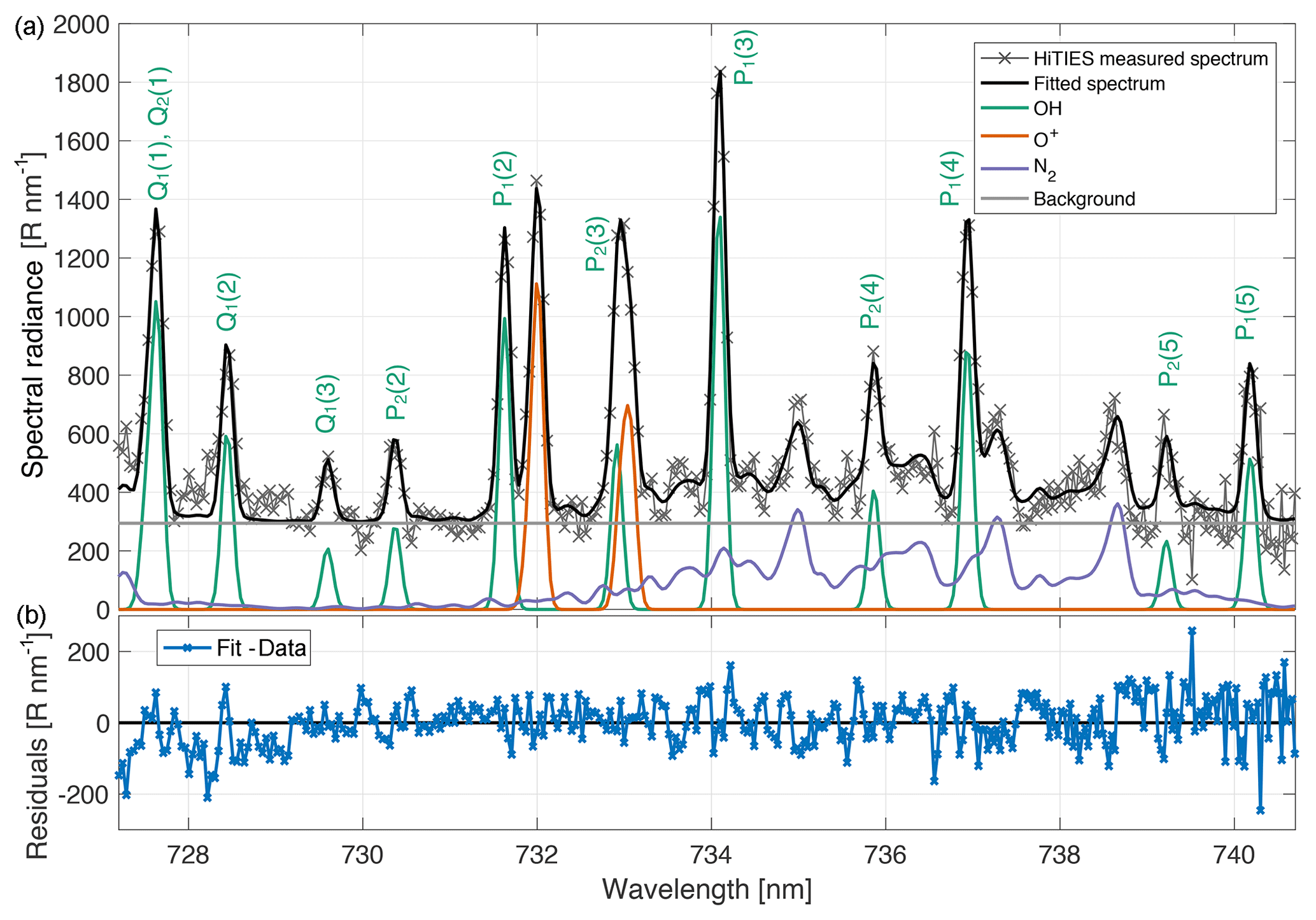
Figure 2 Example HiTIES spectrum during aurora and fitted components (a). The data were taken on 15 December 2015 at 01:40 UT with an integration period of 2 min. The observed spectrum is plotted in light grey with crosses. The fit to the data using the fitting process described in Sect. 4 is shown in a thick black line. The coloured lines represent the components of the fit: OH lines in green, O⁺ in orange, N₂ emission in purple, and the horizontal grey line is a constant background. Panel (b) shows residuals of the fit.

3 Atmospheric emissions

A number of different mosaic filters have been in use with the HiTIES instrument over its years of operation, with filters containing panels observing the wavelength region between 725 and 740 nm in use for most winter seasons since 2003. The spectral fitting described in this paper is applied to spectra in this panel, called the “O⁺ panel”, since it contains two doublets of auroral origin from the O⁺ ion (see Sect. 3.2). The O⁺ panel is located in the top left corner of the four-panel mosaic, as drawn in Fig. 1a, and in the middle of the three-panel mosaic shown in Fig. 1b. Also observed in this panel are OH airglow emissions from the (8-3) Meinel band (see Sect. 3.1) and N₂ 1P emissions from the (6-4) and (5-3) bands (see Sect. 3.3).

An example of a spectrum recorded with the HiTIES O⁺ panel is plotted in Fig. 2a. The observations are shown in grey crosses and the thick black line represents a spectrum that has been fitted to the data using the method described in Sect. 4. The different components of the fit that summed together produce the think black line are plotted in coloured lines: OH lines in green, O⁺ lines in orange, and N₂ band emission in purple.

There are several parameters of interest we aim to retrieve from each HiTIES spectrum that can provide us with information on the state of the upper atmosphere. These parameters are the following:

• intensities of the OH and O⁺ emission lines and of the N₂ emission;

• N₂ rotational temperature;

• OH rotational temperature;

• ratio of O⁺ doublets, which in future will allow for the determination of F-region neutral temperature; and

• precipitable water vapour.

The following, Sect. 3.1 to 3.3, describes the emission components measured by HiTIES in more detail.

3.1 OH airglow

Molecular vibration–rotation transitions in the layer of excited hydroxyl molecules located near the mesopause give rise to airglow emission (Meinel, 1950a, b) that spans from about 500 to 4000 nm (Sigernes et al., 2003). Rocket measurements have shown that the OH layer is centred at approximately 87 km and has a thickness of 8 km (Baker and Stair, 1988). OH airglow emission lines are used to measure the rotational temperature of the molecules at the altitude of emission (Holmen et al., 2014; Phillips et al., 2004; Sigernes et al., 2003). Using the HiTIES instrument, we observe OH lines from the (8-3) vibrational band in the O⁺ panel (Chadney et al., 2017) and from the (5-4) and (9-1) bands in the OH panel.

Hydroxyl rotational temperatures are derived by fitting a straight line to a Boltzmann plot in which $\ln \left\{I/\left[A(\mathrm{2}J+\mathrm{1})\right]\right\}$ is plotted as a function of (hc∕k)F, where I is the OH line intensity, A is the transition probability, J is the upper state total angular momentum quantum number, F is the energy level of the initial rotational level, h is Planck's constant, c is the speed of light, and k is Boltzmann's constant. If we assume a Boltzmann distribution for the rotational level population, the function is linear and the inverse of the slope of the fitted straight line is the neutral temperature. An example of a Boltzmann plot can be found in Fig. 3. In determining the temperature, we make use of the strongest P-branch OH(8–3) lines recorded by HiTIES, the four P₁ lines: P₁(2), P₁(3), P₁(4), and P₁(5). These are shown in blue circles in Fig. 3; see also these lines labelled in the spectrum in Fig. 2. As LTE is not always assured, especially in the higher vibrational states of OH (Pendleton et al., 1993), we place constraints on the variance between the linear fit and the P₁ and P₂ lines (the latter are the red circles in Fig. 3). A given temperature retrieval is rejected if the linear fit to P₁ line variance is greater than 0.05 or if the linear fit to P₂ line variance is over 0.3. For more information on this process, see Chadney et al. (2017).

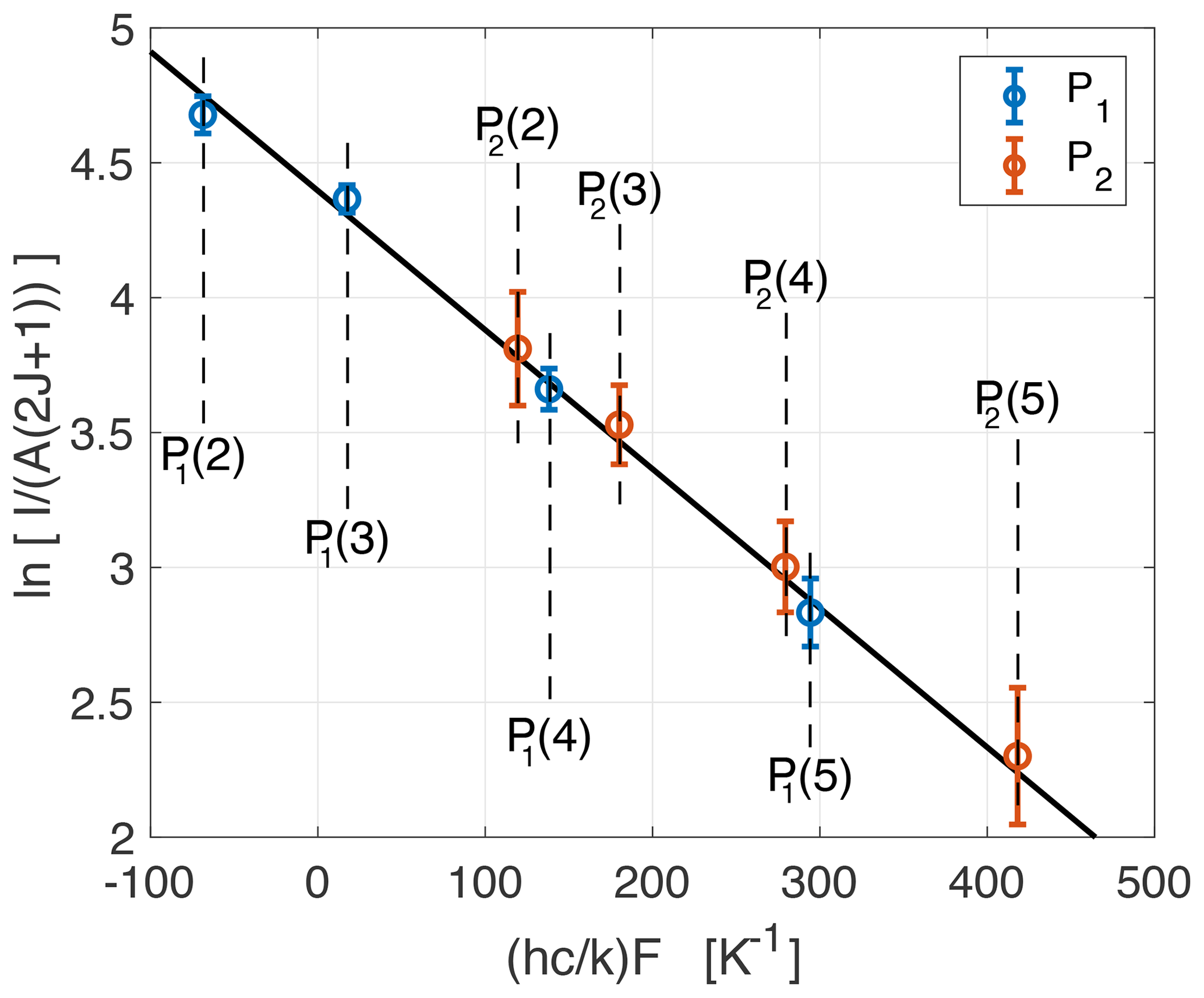
Figure 3 Boltzmann plot determined from the OH(8-3) P-branch lines shown in the HiTIES spectrum from Fig. 2, taken on the 15 December 2015 at 01:40 UT with an integration time of 2 min. The solid black line is a linear fit to the P₁ lines (shown as blue circles); the inverse of the slope gives a rotational temperature of 193.9 K. Errors on the OH intensities I are obtained from the residuals of the spectral fit.

Water vapour in the troposphere is responsible for absorbing each of the OH lines to a different degree; of the OH lines measured in the HiTIES O⁺ panel, the OH(8-3) P₁(4) line at 736.9 nm is particularly affected by H₂O absorption, which must thus be taken into account to accurately determine the OH rotational temperature. Therefore, we model water vapour absorption using the HIgh-resolution TRANsmission molecular absorption database, HITRAN (Rothman et al., 2013), in order to remove its effect from the measured OH line intensities. This process, which is described further in Sect. 4 and Chadney et al. (2017), also provides us with an estimate of the column density of water vapour in the atmosphere: the precipitable water vapour (PWV).

3.2 O⁺ aurora

The O⁺ panel is so named because it contains two spectrally unresolved emission line doublets from the O⁺ ion at 731.904 and 732.012 and at 732.968 and 733.076 nm (Sharpee et al., 2004) resulting from the transitions ${}^{\mathrm{2}}{P}_{\mathrm{1}/\mathrm{2},\mathrm{3}/\mathrm{2}}^{\mathrm{0}}\to$ ${}^{\mathrm{2}}{D}_{\mathrm{5}/\mathrm{2}}^{\mathrm{0}}$ and ${}^{\mathrm{2}}{P}_{\mathrm{1}/\mathrm{2},\mathrm{3}/\mathrm{2}}^{\mathrm{0}}\to$ ${}^{\mathrm{2}}{D}_{\mathrm{3}/\mathrm{2}}^{\mathrm{0}}$, respectively. These emission doublets are shown in orange in the spectrum of Fig. 2. Electron impact ionisation from low-energy precipitating electrons produces the excited O⁺ states that are responsible for the auroral O⁺ emission measured by HiTIES. Furthermore, the ratio of the two O⁺ doublets $R_{{\mathrm{O}}^{+}}=(I_{\mathrm{731.904}\mathrm{nm}}+I_{\mathrm{732.012}\mathrm{nm}})/(I_{\mathrm{732.968}\mathrm{nm}}+I_{\mathrm{733.076}\mathrm{nm}})$ is of particular interest. Indeed, Whiter et al. (2014) showed that the value of $R_{{\mathrm{O}}^{+}}$ depends on the neutral temperature, thus allowing for a measurement of T_n at the high altitudes at which the O⁺ emission is produced (∼250 km). Further validation is needed to convert $R_{{\mathrm{O}}^{+}}$ to T_n, so in the remainder of this paper, we will only consider the ratio $R_{{\mathrm{O}}^{+}}$.

3.3 N₂ aurora

N₂ first positive (1P) emission is measured in the HiTIES O⁺ panel. With the four-panel mosaic (depicted in Fig. 1a), it is mostly the (5-3) band that is observed since the band head wavelength is 738.72 nm and N₂ 1P bands are degraded to the violet. With the newer three-panel mosaic (Fig. 1b), the extended wavelength range of the O⁺ panel means that portions of the (4-2) and (6-4) bands, with band head wavelengths of 750.47 and 727.40 nm, respectively, are also observed. The N₂ 1P component of the fit to the HiTIES spectrum in Fig. 2 is shown in purple.

Following the methods of Jokiaho et al. (2008, 2009), synthetic N₂ 1P line spectra are produced for vibrational levels 0 to 12 at different rotational temperatures. These spectra are convolved with a Gaussian instrument function of full width at half maximum (FWHM) equal to 0.12 nm to produce the synthetic N₂ 1P spectra plotted in Fig. 4. The clear change in spectral shape with rotational temperature allows us to retrieve a value for the N₂ rotational temperature by choosing the best fit synthetic spectrum to a given HiTIES measurement (see Sect. 4). Future analysis of the dataset of N₂ temperatures will consider the conditions under which the layer can be considered in LTE.

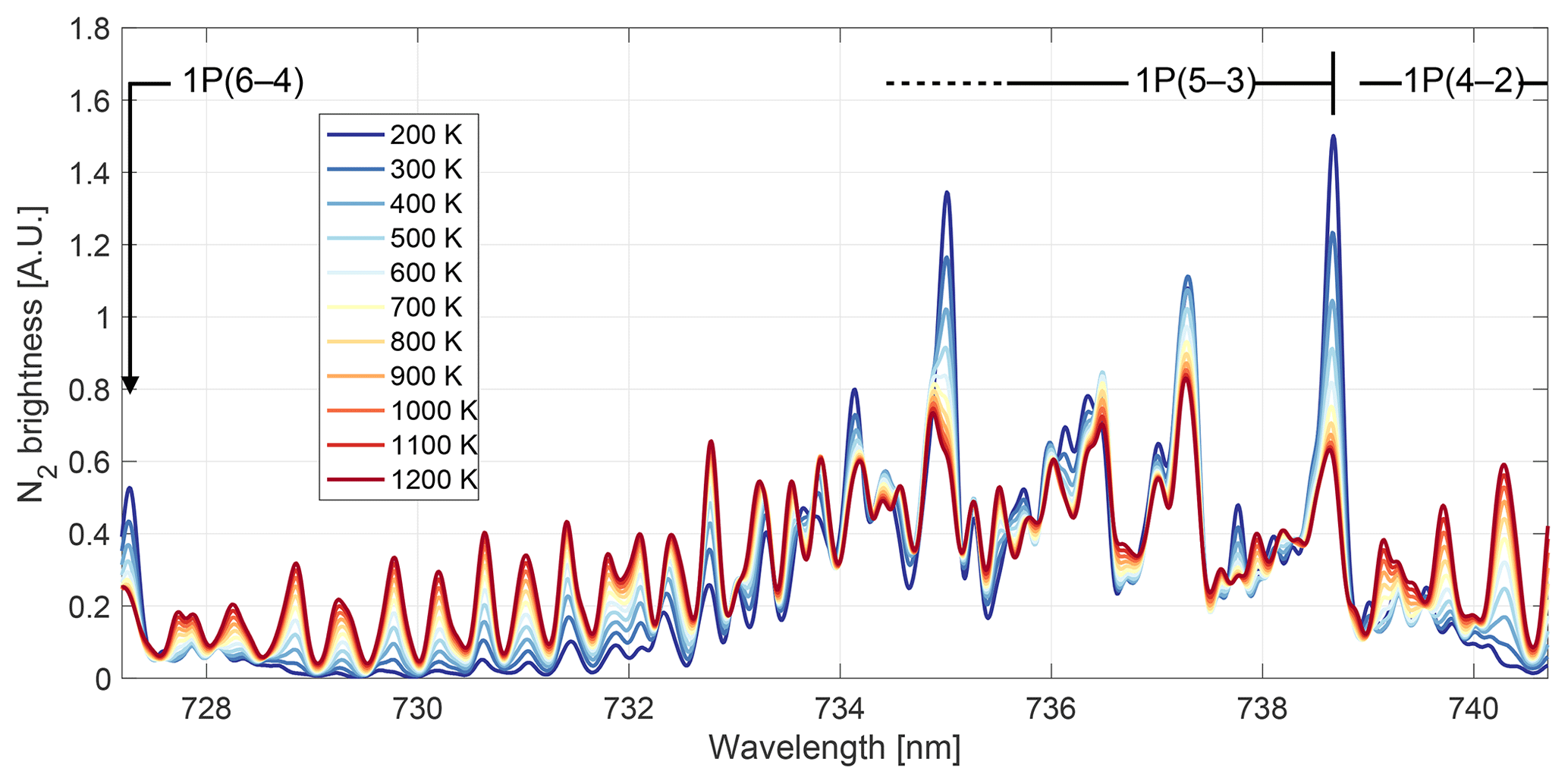
Figure 4 Synthetic N₂ spectra at different rotational temperatures. The rotational band and, where present, band heads are labelled above the spectra.

4 Fitting process

A least-squares fitting routine is used to determine the parameters of the superposed emissions present in the measured HiTIES spectra. The OH and O⁺ lines are represented as Gaussians, all with the same FWHM, since the width is principally determined by the instrument function. Line centre wavelengths are fixed at the values given in Table 1. OH rotational states are split due to nuclear-spin–electron-orbit interactions, referred to as Λ doubling. The resulting Λ-doubled components are not spectrally resolved by HiTIES, meaning that the hydroxyl emission lines in Fig. 2 are made up of two components, labelled with the subscripts e and f (referring to the parity of the lower state) in Table 1. We fit a Gaussian for each Λ-doubled component and make the assumption that the two components of each OH vibrational–rotational transition are of equal intensity; thus we fix the peak height of the Gaussian representing the f component of each transition to have the same peak height as the e component.

The two O⁺ doublets are represented in the fit by four Gaussians centred at the wavelengths given in Table 1. From the Einstein coefficients of these transitions (Zeippen, 1987), we obtain the following constraints on the intensities of the O⁺ lines:

$$\begin{array}{}\text{(1)}& {\displaystyle }I{(}^{\mathrm{2}}{\mathrm{P}}_{\mathrm{1}/\mathrm{2}}^{\mathrm{0}}\to {}^{\mathrm{2}}{\mathrm{D}}_{\mathrm{3}/\mathrm{2}}^{\mathrm{0}})=\mathrm{1.668}\times I{(}^{\mathrm{2}}{\mathrm{P}}_{\mathrm{1}/\mathrm{2}}^{\mathrm{0}}\to {}^{\mathrm{2}}{\mathrm{D}}_{\mathrm{5}/\mathrm{2}}^{\mathrm{0}}),\text{(2)}& {\displaystyle }I{(}^{\mathrm{2}}{\mathrm{P}}_{\mathrm{3}/\mathrm{2}}^{\mathrm{0}}\to {}^{\mathrm{2}}{\mathrm{D}}_{\mathrm{3}/\mathrm{2}}^{\mathrm{0}})=\mathrm{0.540}\times I{(}^{\mathrm{2}}{\mathrm{P}}_{\mathrm{3}/\mathrm{2}}^{\mathrm{0}}\to {}^{\mathrm{2}}{\mathrm{D}}_{\mathrm{5}/\mathrm{2}}^{\mathrm{0}}),\end{array}$$

where I is the line intensity. Equations (1) and (2) are included as constraints in the fitting process, allowing for 10 % variation in the coefficients.

We create a database of N₂ model spectra at temperatures from 150 to 1150 K, with a resolution of 10 K and an instrument function FWHM appropriately chosen for the focus of the HiTIES instrument during a given season. The fitting routine finds the best match to the data out of this grid of modelled spectra, providing a direct retrieval of the N₂ rotational temperature.

Each measured HiTIES spectrum is fitted with 30 parameters: 24 OH line peak intensities (modelled as 48 Gaussians with e and f components constrained to have the same height for the same rotational–vibrational transition), two O⁺ line intensities (modelled as four Gaussians, with constrained ratios between the upper and lower wavelength components of each doublet given in Eqs. 1 and 2), the FWHM (assumed the same for all the OH and O⁺ Gaussians), the intensity and rotational temperature of the N₂ emission, and a constant background intensity. Figure 2a shows the resulting fit to a spectrum recorded by HiTIES on 15 December 2015 at 01:40 UT; the data are shown in light grey and the fitted spectrum is a thick black line. Figure 2b shows the residuals of this fit, for which it can be seen that a good fit to the data is achieved with the chosen parameters. However, at the short wavelength end of the spectrum, there are a few emission features in the data that are not present in the fitted spectrum, in particular peaks near 727.3, 728.0, and 728.9 nm. We believe these peaks correspond to O₂ emission, which is not included in our fit. Therefore, our fitted values of the Q-branch OH(8-3) lines, present at the short wavelength end of the HiTIES spectrum, are likely unreliable, so these OH lines are not used for the temperature retrieval.

With the fitted intensities of the P-branch OH lines, we determine the OH rotational temperature by constructing a Boltzmann plot (see Sect. 3.1 and Fig. 3). The temperature retrieval is performed using the strongest P₁ branch lines: P₁(2), P₁(3), P₁(4), and P₁(5).

Tropospheric water vapour absorption attenuates many of the emission lines measured with HiTIES. This effect must be taken into account for correct parameter retrieval from the fitting process. Modelling of the H₂O absorption in each line is not just done for OH emission, as described in Sect. 3.1, but also for each O⁺ and N₂ emission line. The HITRAN (Rothman et al., 2013) spectral database is used to determine the H₂O absorption cross section, and water vapour absorption in the column of atmosphere above the instrument is calculated using the Beer–Lambert law (Chadney et al., 2017). We parameterise water vapour absorption with the coefficient ς given for the OH and O⁺ lines in Table 1, which is related to absorption (a_λ) and transmission (t_λ) coefficients by the following:

$$\begin{array}{}\text{(3)}& t_{\mathit{\lambda }}=\mathrm{1}-a_{\mathit{\lambda }}=\exp \left(-\mathit{\varsigma }\times \mathrm{PWV}\right),\end{array}$$

where PWV is the precipitable water vapour in millimetres. PWV represents the height of a column of liquid water that would result from the condensation of all the water in a column of atmosphere. Thus, a PWV of 1 mm is equivalent to a column density of H₂O of 1 kg m⁻².

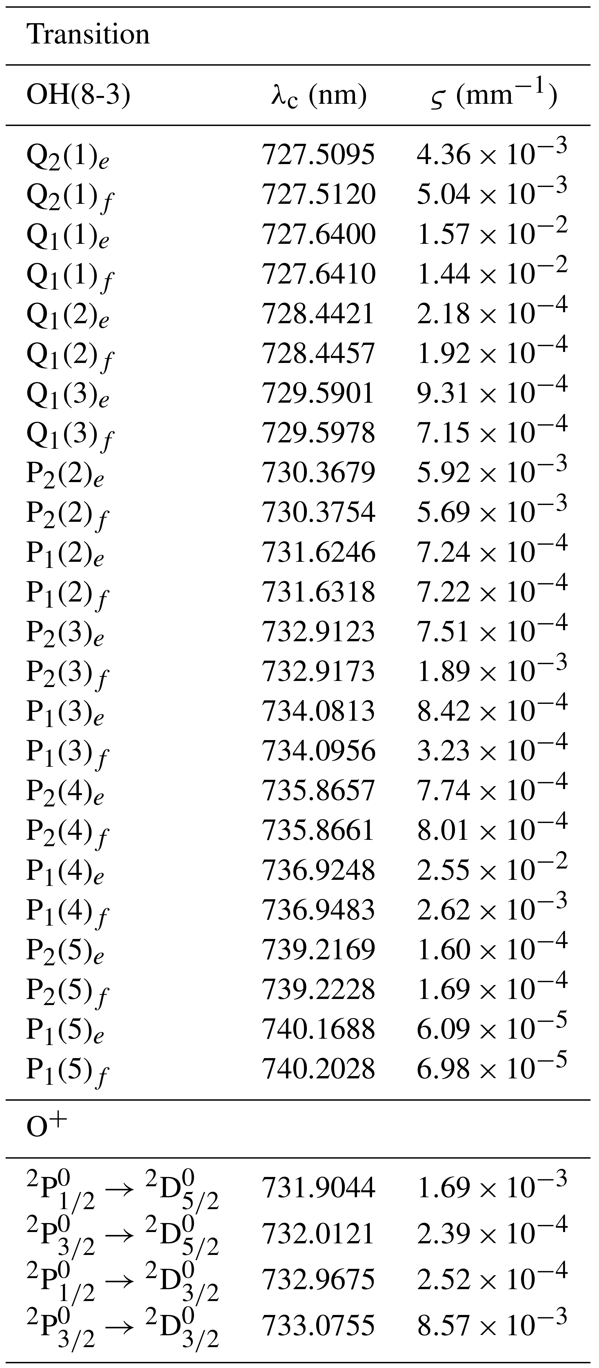
Table 1 Emission lines used in the spectral fit. The line centre wavelengths (λ_c) are from Rousselot et al. (2000), converted to air wavelengths following Ciddor (1996). Water vapour transmission is given by a function of PWV: $t_{\mathit{\lambda }}=\exp (-\mathit{\varsigma }\times \mathrm{PWV})$, with PWV in millimetres.

The spectral fitting and OH temperature retrieval process is run multiple times, each assuming a different given value of PWV. From the Boltzmann plot constructed with OH P-branch lines, the correlation coefficient R² of the linear fit allowing for temperature retrieval is determined for each of these runs. The retrieved value of PWV for a given HiTIES spectrum is then taken as the PWV that maximises the Boltzmann plot correlation coefficient R². An example of this process is shown in Fig. 5 for the spectrum from Fig. 2, taken on 15 December 2015 at 01:40 UT. Each blue point in Fig. 5 is a value of R² from a Boltzmann plot constructed using the OH P-branch line intensities calculated by the spectral fitting routine, assuming a given value of the PWV between 0 and 10 mm. The value of PWV which maximises R² is found by fitting the blue points in Fig 5. Since water vapour absorption is calculated using the Beer–Lambert law, which takes the form of an exponential, we find that the expression that provides the best fit to the R² points is a sum of exponentials,

$$\begin{array}{}\text{(4)}& R^{\mathrm{2}}=a\exp \left(b\times \mathrm{PWV}\right)+c\exp \left(d\times \mathrm{PWV}\right),\end{array}$$

and thus the maximum of R² is attained at a precipitable water vapour of

$$\begin{array}{}\text{(5)}& \mathrm{PWV}={\displaystyle \frac{\mathrm{1}}{b-d}}\ln \left(-{\displaystyle \frac{cd}{ab}}\right).\end{array}$$

To reduce computational time, we have found that it is sufficient to run the retrieval process at just five different values of PWV in order to determine the maximum of R².

Figure 5 Correlation coefficient R² to a straight line in the Boltzmann plot as a function of PWV used to correct the OH line intensities from the HiTIES spectrum recorded on 15 December 2015 at 01:40 UT (from Fig. 2). The blue points are values of R² produced by the fitting process for each assumed value of PWV. The red curve is a fit to these points and is used to determine the PWV at which R² peaks.

Considering that the main source of noise in a given spectrum is shot noise, we determine the uncertainties on the fitted line intensities (e_I) using the following:

$$\begin{array}{}\text{(6)}& e_{\mathrm{I}}={\mathit{\sigma }}_{\mathrm{residuals}}\times \sqrt{N_{\mathrm{pixels}}},\end{array}$$

where σ_residuals is the standard deviation of the residuals and N_pixels is the number of pixels on the detector contained in the FWHM of the emission line. In this way, we can obtain uncertainty estimates on the parameters retrieved from each particular spectrum. However, we would also like to determine the ranges of parameters over which the fitting process produces accurate results. For this reason, we carry out a Monte Carlo simulation in Sect. 5.

5 Parameter retrieval tests

In order to estimate expected errors on the fitting and parameter retrieval process described in Sect. 4, we have performed a Monte Carlo simulation. Such a simulation also provides information on the region of parameter space over which the fitting method is valid. Synthetic spectra were generated containing OH, O⁺, and N₂ components in different proportions and with different properties. The parameters of each synthetic spectrum were drawn randomly within the following ranges.

• $I_{\mathrm{OH}}^{\mathrm{in}}\equiv I_{{\mathrm{OHP}}_{\mathrm{1}}\left(\mathrm{3}\right)}^{\mathrm{in}}=\mathrm{1300}$ R nm⁻¹

• $T_{\mathrm{OH}}^{\mathrm{in}}\in \left[\mathrm{170},\mathrm{240}\right]$ K

• $I_{{\mathrm{N}}_{\mathrm{2}}}^{\mathrm{in}}\equiv \max \left(I_{{\mathrm{N}}_{\mathrm{2}}}^{\mathrm{in}}\left(\mathit{\lambda }\right)\right)\in \left[\mathrm{0},\mathrm{3900}\right]$ R nm⁻¹

• $T_{{\mathrm{N}}_{\mathrm{2}}}^{\mathrm{in}}\in \left[\mathrm{180},\mathrm{1000}\right]$ K

• $I_{{\mathrm{O}}^{+}}^{\mathrm{in}}\equiv I_{{\mathrm{O}}^{+}\mathrm{732}\mathrm{nm}}^{\mathrm{in}}\in \left[\mathrm{0},\mathrm{3900}\right]$ R nm⁻¹

• $R_{{\mathrm{O}}^{+}}^{\mathrm{in}}\in \left[\mathrm{1.25},\mathrm{1.4}\right]$

• $I_{\mathrm{back}}^{\mathrm{in}}=\mathrm{300}$ R nm⁻¹

• ${\mathrm{PWV}}^{\mathrm{in}}\in \left[\mathrm{0},\mathrm{20}\right]$ mm

Note that I_OH represents the intensity of the strongest OH line measured by HiTIES, the OH(8-3) P₁(3) line; $I_{{\mathrm{O}}^{+}}$ is the intensity of the O⁺ doublet at 732 nm, the intensity of the N₂ emission, $I_{{\mathrm{N}}_{\mathrm{2}}}$, is the maximum intensity of this emission over the 728 to 740 nm range, and I_back is the level of the background emission. We use the superscript “in” to mean parameters that are used to construct the synthetic spectra (inputs to the MC simulation or theoretical values) and the superscript “ret” for the value of parameters retrieved from the spectral fitting process. The values of $I_{\mathrm{OH}}^{\mathrm{in}}$ and $I_{\mathrm{back}}^{\mathrm{in}}$ are fixed to values consistent with those from the HiTIES spectrum plotted in Fig. 2.

In constructing the synthetic spectra, we add random noise to the intensity values in each wavelength bin. This random noise follows a Gaussian distribution with standard deviation $\sqrt{I}$ in each bin to simulate shot noise. Since HiTIES uses an electron multiplying charge-coupled device (EMCCD), there is no read-out noise. For the simulations presented in Sects. 5.1–5.5 and 6, we neglect thermal noise as the detector is cooled to −80 ^∘C (see Sect. 5.6 for a brief discussion of the validity of this assumption). In all, 50 000 synthetic spectra are produced and run through the fitting and temperature retrieval process. This number is sufficient to ensure convergence of the Monte Carlo simulation.

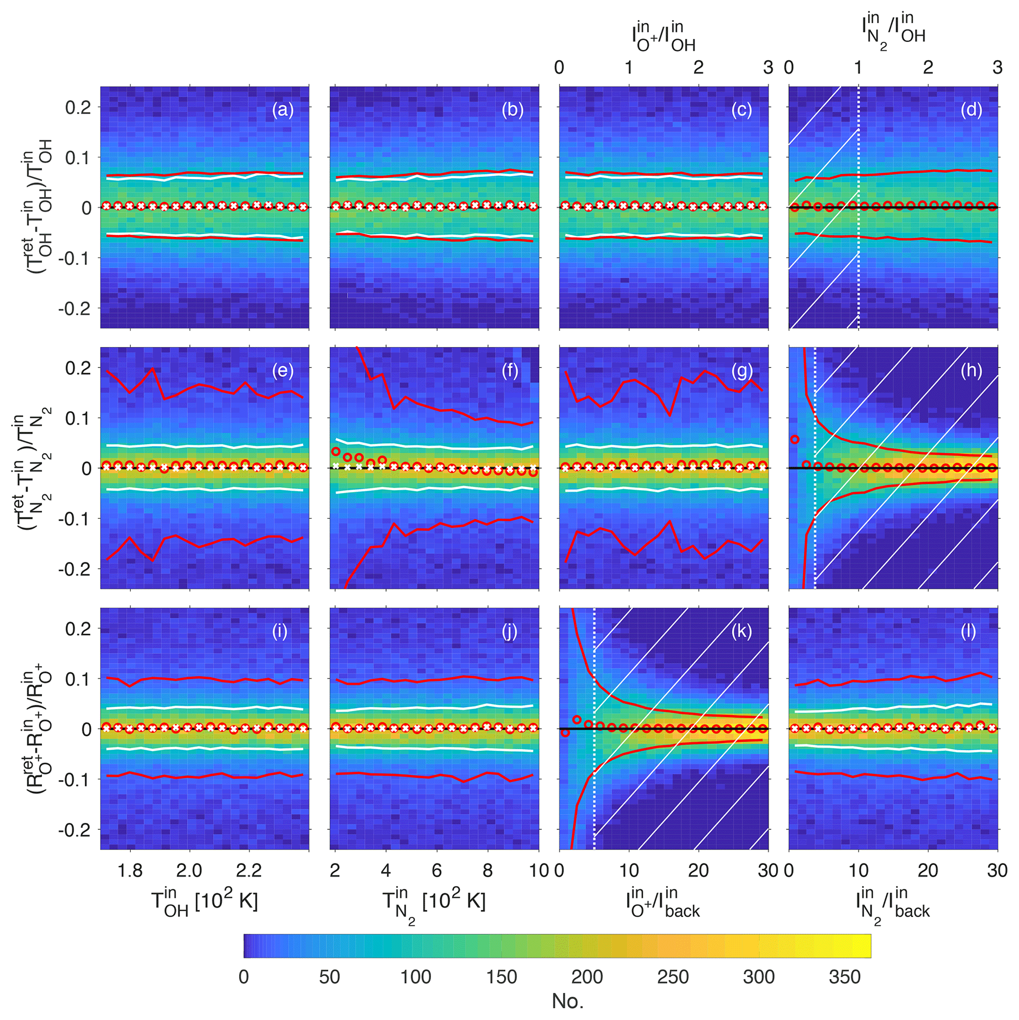
Figure 6 2-D histograms of parameter retrieval tests using 50 000 synthetic spectra. (a, b, c, d) The fractional error on the retrieval of the OH temperature T_OH, (e, f, g, h) the error on the N₂ temperature, $T_{{\mathrm{N}}_{\mathrm{2}}}$, and (i, j, k, l) the error on the O⁺ ratio $R_{{\mathrm{O}}^{+}}$. Panels (c, g, k) and (d, h, l) show the errors as a function of the input O⁺ and N₂ intensities, respectively. These intensities are normalised by either the OH intensity or the intensity of the background I_back. Red circles indicate mean values and red lines show 1 standard deviation on either side of the mean using all of the generated synthetic spectra. (a, b, c) White crosses and thick white lines are mean values and 1 standard deviation from the mean, respectively, when the N₂ intensity parameter space is restricted to the hatched area in panel (d). Similarly, the white crosses and lines in panels (e, f, g) represent the mean and 1 standard deviation from the mean, respectively, including only spectra with N₂ intensities within the hatched area in panel (h). The white crosses and dotted lines in panels (i, j, l) are the mean and 1 standard deviation, respectively, including only spectra with O⁺ intensities in the hatched area in panel (k).

By comparing the input parameters to those retrieved, we assess how well the spectral fitting method described in Sect. 4 can extract the different parameters of a HiTIES spectrum. The main results of this process are plotted as two-dimensional histograms in the panels of Fig. 6. Each row of this plot shows the error on the retrieval of a parameter of interest. The top row, made up of panels (a, b, c, d), represents fractional errors on the retrieval of the OH temperature as a function of the theoretical OH temperature of the synthetic spectrum, $T_{\mathrm{OH}}^{\mathrm{in}}$, the theoretical N₂ temperature, $T_{{\mathrm{N}}_{\mathrm{2}}}^{\mathrm{in}}$, the intensity of O⁺, and the intensity of N₂, respectively. The middle row (Fig. 6e, f, g, h) contains plots showing the fractional error on the retrieval of the N₂ temperature, and plots in the bottom row, panels (i, k, j, l), show the fractional error on the retrieval of the ratio between the intensities of the O⁺ doublets, $R_{{\mathrm{O}}^{+}}$. The intensities of the different emissions vary enormously between spectra recorded at different times. Therefore, the intensities of O⁺ and N₂ that we have plotted along the x axis of panels (c, g, k) and (d, h, l), respectively, are normalised by the intensity of the OH(8-3) P₁(3) line, $I_{\mathrm{OH}}^{\mathrm{in}}$, and the intensity of the background, $I_{\mathrm{back}}^{\mathrm{in}}$, as $I_{\mathrm{OH}}^{\mathrm{in}}$ and $I_{\mathrm{back}}^{\mathrm{in}}$ have values that are fixed in all synthetic spectra.

The histograms that make up each panel of Fig. 6 are constructed with the 50 000 synthetic spectra that have been processed using the spectral fitting routine. The red circle markers show the mean values and the red lines represent 1 standard deviation on either side of the mean, obtained when dividing the x axes into 18 equally sized bins. In some cases it is possible to significantly lower the standard deviation by applying a threshold on one of the parameters to reduce the sample of synthetic spectra chosen. For example, one would not expect to be able to measure the N₂ temperature if there is little to no emission from this molecule in the spectrum, so it makes sense to impose a minimum value on $I_{{\mathrm{N}}_{\mathrm{2}}}^{\mathrm{in}}$ for the retrieval of $T_{{\mathrm{N}}_{\mathrm{2}}}$. For each row of plots in Fig. 6 the white vertical dotted line and associated hatched area in the panel in either the third column (for the bottom row) or fourth column (for the top and middle rows) represents the threshold applied on the intensity of O⁺ or N₂ used to reduce the standard deviations in the other panels of each row. The lower standard deviations of the reduced samples are shown with white lines in panels (a, b, c) for the error on the retrieval of T_OH (only considering spectra with $I_{{\mathrm{N}}_{\mathrm{2}}}^{\mathrm{in}}<\mathrm{1}\times I_{\mathrm{OH}}^{\mathrm{in}}$), in panels (e, f, g) for the retrieval of $T_{{\mathrm{N}}_{\mathrm{2}}}$ (only considering spectra with $I_{{\mathrm{N}}_{\mathrm{2}}}^{\mathrm{in}}>\mathrm{3.7}\times I_{\mathrm{back}}^{\mathrm{in}}$), and in panels (i, j, l) for the retrieval of $R_{{\mathrm{O}}^{+}}$ (only considering spectra with $I_{{\mathrm{O}}^{+}}^{\mathrm{in}}>\mathrm{5}\times I_{\mathrm{back}}^{\mathrm{in}}$). The following sections describe the results of the Monte Carlo simulation with regards to the retrieval of each atmospheric parameter of interest.

5.1 Retrieval of OH temperature

The fractional error on the retrieval of OH temperature, $\left(T_{\mathrm{OH}}^{\mathrm{ret}}-T_{\mathrm{OH}}^{\mathrm{in}}\right)/T_{\mathrm{OH}}^{\mathrm{in}}$, is shown in Fig. 6a, b, c, and d. The bias, shown with red circle markers, is very close to being 0, with a standard deviation that varies between 5 % and 8 %. If we apply a maximum threshold of $I_{{\mathrm{N}}_{\mathrm{2}}}^{\mathrm{in}}=\mathrm{1}\times I_{\mathrm{OH}}^{\mathrm{in}}$, represented by the white dotted vertical line in panel (d), the standard deviation is reduced to between 5 % and 6 %, with no dependence on $T_{\mathrm{OH}}^{\mathrm{in}}$, $T_{{\mathrm{N}}_{\mathrm{2}}}^{\mathrm{in}}$, or $I_{{\mathrm{O}}^{+}}^{\mathrm{in}}$, as indicated by the white dotted lines in panels (a), (b), and (c). Indeed, the red lines in panel (d) show that the spread of errors on the retrieval increases slightly with the N₂ intensity. This makes sense since the band structure of N₂ emission means that it is present in all wavelength bins of the HiTIES detector (see Fig. 4); therefore, at high levels of N₂ emission it is more difficult to distinguish the precise height of the OH lines, with a standard deviation on the error of T_OH retrieval of almost 8 % when $I_{{\mathrm{N}}_{\mathrm{2}}}^{\mathrm{in}}=\mathrm{3}\times I_{\mathrm{OH}}^{\mathrm{in}}$.

The uncertainties stated here are for a single temperature measurement. However, HiTIES is capable of providing at least one such observation every 2 min, as long as there are OH lines being recorded, which is the case the vast majority of the time that the instrument is running. Therefore, with temporal averaging it is possible to reduce the size of the errors. If one assumes a typical OH temperature of 200 K, the relative uncertainty of 6 % revealed by our Monte Carlo simulation translates to an absolute uncertainty of σ=12 K. Averaging over N=5 measurements (representing a time resolution of 10  min if the individual spectra are integrated over 2 min of observation time) reduces the absolute uncertainty to $\mathit{\sigma }/\sqrt{N}=\mathrm{5.4}$ K. Similarly, temporal averaging over N=15 observations would reduce the absolute uncertainty on the measured OH temperature to $\mathit{\sigma }/\sqrt{N}=\mathrm{3.1}$ K, with a possible time resolution of 30 min.

5.2 Retrieval of N₂ temperature

The fractional error on the retrieval of N₂ temperature, $\left(T_{{\mathrm{N}}_{\mathrm{2}}}^{\mathrm{ret}}-T_{{\mathrm{N}}_{\mathrm{2}}}^{\mathrm{in}}\right)/T_{{\mathrm{N}}_{\mathrm{2}}}^{\mathrm{in}}$, is shown in Fig. 6e, f, g, and h. The bias on the retrieval is almost 0 for most values of the input parameters shown on the x axes of these panels, as indicated by the red circle markers. The standard deviations taking into account all 50 000 synthetic spectra, shown in red lines, are large and very variable, which is due to the inclusion of spectra for which there is no (and very little) N₂ emission – it is not possible to obtain a temperature measurement in these cases. If we impose a minimum value on the intensity of N₂ emission of $I_{{\mathrm{N}}_{\mathrm{2}}}^{\mathrm{in}}=\mathrm{3.7}\times I_{\mathrm{back}}^{\mathrm{in}}$ (vertical white dotted line in panel h), we can lower the standard deviation on the fractional error of $T_{{\mathrm{N}}_{\mathrm{2}}}^{\mathrm{in}}$ retrieval to between 3 % and 5 %. The cut-off value of $\mathrm{3.7}\times I_{\mathrm{back}}^{\mathrm{in}}$ is chosen as the location in panel (h) at which the standard deviation dips below 10 %.

The very high standard deviations at low N₂ temperatures seen in panel (f) are due to the fact that the initial value of $T_{{\mathrm{N}}_{\mathrm{2}}}$ in the spectral fitting is set at the lowest temperature. Therefore, the retrievals included in the left portion of the 2-D histogram include many spectra with little to no N₂ emission. Indeed, once the lowest values of $I_{{\mathrm{N}}_{\mathrm{2}}}$ are eliminated, the standard deviation is reduced to about 5 % (as shown by the white lines), with little dependency on $T_{{\mathrm{N}}_{\mathrm{2}}}$.

Panel (f) shows a dependency of the bias on $T_{{\mathrm{N}}_{\mathrm{2}}}$ when all 50 000 spectral retrievals are considered. The red circle markers indicate that there is a bias towards overestimating the lowest N₂ temperatures and underestimating the highest. Because of the very large spread of retrieved temperatures, the mean values are skewed at the edges of the temperature domain. This bias on the mean is eliminated by the reduction of the standard deviation on the temperature uncertainties when imposing a minimum threshold on $I_{{\mathrm{N}}_{\mathrm{2}}}$; the white crosses representing the mean values in this case are all on the line of zero error.

5.3 Retrieval of O⁺ doublet ratio

The fractional error on the retrieval of the intensity ratio of the two O⁺ doublets, $\left(R_{{\mathrm{O}}^{+}}^{\mathrm{ret}}-R_{{\mathrm{O}}^{+}}^{\mathrm{in}}\right)/R_{{\mathrm{O}}^{+}}^{\mathrm{in}}$, is shown in the Fig. 6i, j, k, and l. The ratio $R_{{\mathrm{O}}^{+}}=I_{{\mathrm{O}}^{+}\mathrm{732}\mathrm{nm}}^{\mathrm{in}}/I_{{\mathrm{O}}^{+}\mathrm{733}\mathrm{nm}}^{\mathrm{in}}$ can only be measured when there is sufficient O⁺ emission present in the spectrum to distinguish it from the background. This effect can be seen in panel (k), in which the red lines show that the standard deviation on the mean becomes very high as $I_{{\mathrm{O}}^{+}}^{\mathrm{in}}\to \mathrm{0}$. Taking a minimum threshold on the intensity of O⁺ emission of $I_{{\mathrm{O}}^{+}}^{\mathrm{in}}=\mathrm{5}\times I_{\mathrm{back}}^{\mathrm{in}}$ brings the standard deviation on the mean below 5 %. The minimum threshold value is shown by the white vertical dotted line in panel (k) of Fig. 6.

The error on the retrieval of $R_{{\mathrm{O}}^{+}}$ does not depend on either T_OH or $T_{{\mathrm{N}}_{\mathrm{2}}}$. There is a slight dependency on $I_{{\mathrm{N}}_{\mathrm{2}}}$, with the spread of errors being larger when there is more intense N₂ emission.

5.4 Retrieval of OH intensity

Figure 7 shows 2-D histograms of the fractional error on the retrieval of the intensity of OH, $\left(I_{\mathrm{OH}}^{\mathrm{ret}}-I_{\mathrm{OH}}^{\mathrm{in}}\right)/I_{\mathrm{OH}}^{\mathrm{in}}$, as a function of the intensity of O⁺ in panel (a) and the intensity of N₂ in panel (b). As in Fig. 6, the red circle markers in Fig. 7 represent the mean values and the red lines are 1 standard deviation on either side of the mean for all 50 000 synthetic spectra. The white lines in panel (a) are the standard deviation on either side of the mean when only considering spectra with $I_{{\mathrm{N}}_{\mathrm{2}}}^{\mathrm{in}}<\mathrm{1}\times I_{\mathrm{OH}}^{\mathrm{in}}$. This threshold is indicated by the vertical white dotted line and hatched area in panel (b).

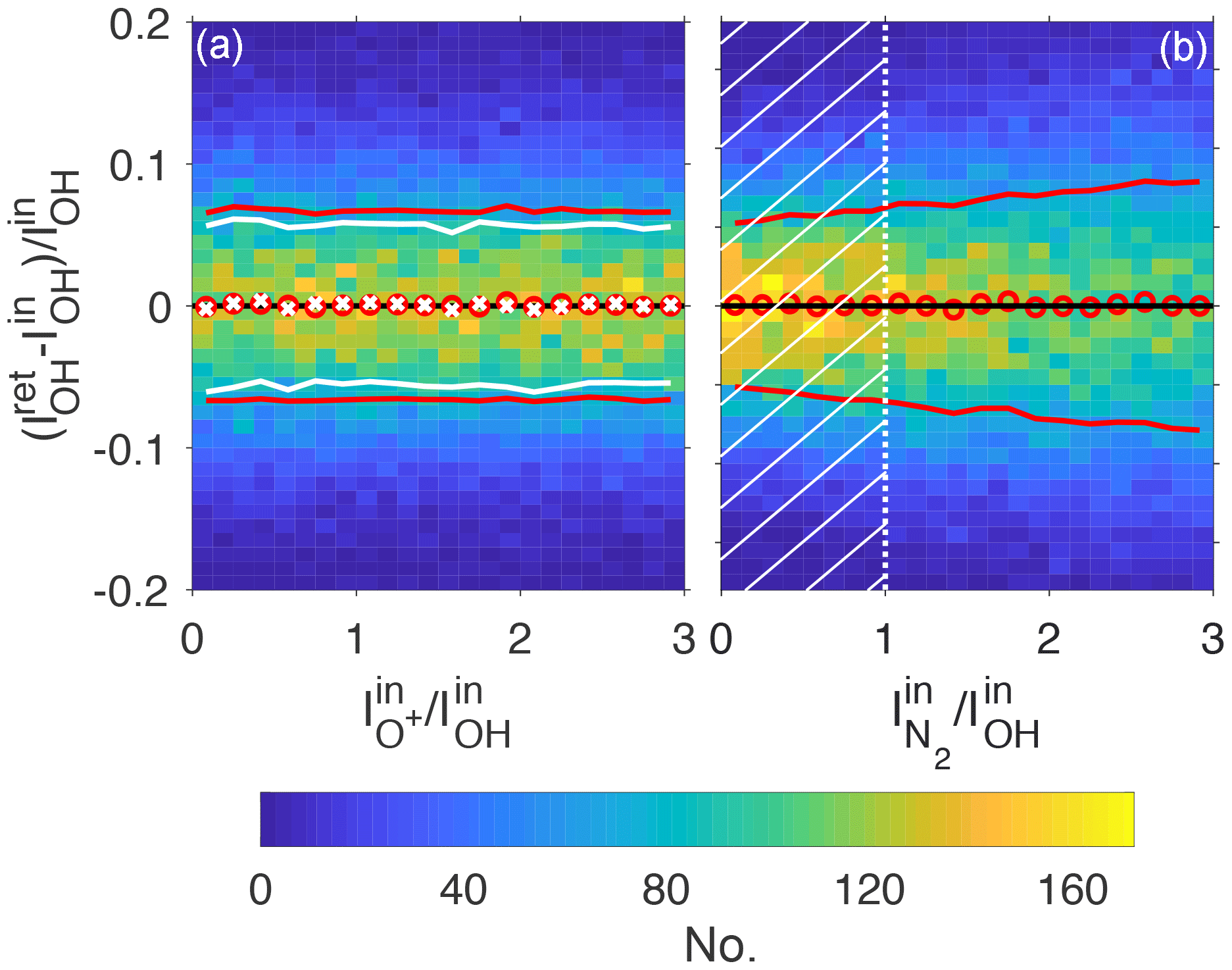
Figure 7 2-D histograms of errors on the retrieval of OH intensity as a function of the ratio of O⁺ to OH intensity (a) and as a function of the ratio of N₂ to OH intensity (b). Red circles indicate mean values and red lines are 1 standard deviation on either side of the mean. The white crosses and lines in panel (a) represent the mean and 1 standard deviation from the mean when only taking into account spectra with N₂ intensity in the hatched area in panel (b).

Figure 7a shows that there is no dependency of the error on the intensity of O⁺; i.e. O⁺ emission does not impede the retrieval of the OH intensity. The standard deviation can be reduced from about 7 % to 5 %–6 % by imposing the maximum threshold described above on the N₂ intensity, since there is a slight dependence of the I_OH retrieval error on $I_{{\mathrm{N}}_{\mathrm{2}}}$ (see Fig. 7b).

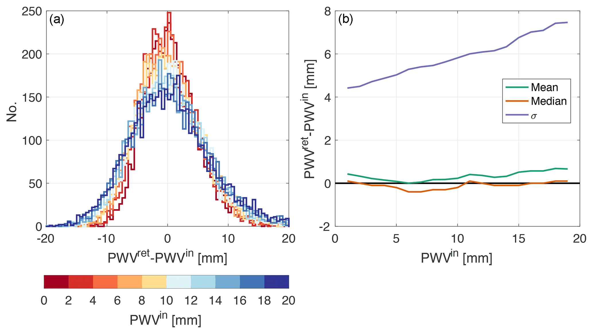
Figure 8 Errors on the retrieval of PWV. (a) Stacked histograms of the difference between the retrieved value, PWV^ret, and the theoretical value used to construct the synthetic spectrum, PWVⁱⁿ, separated into different ranges of PWVⁱⁿ. (b) The mean values (in green), the median (in orange), and the standard deviation σ (in purple) for the same ranges of PWVⁱⁿ as in (a).

5.5 Retrieval of precipitable water vapour

Another parameter of interest to retrieve from HiTIES spectra is the density of water vapour present in the column of atmosphere above the instrument. Values of precipitable water vapour (PWV) are obtained by comparing the absorption of OH lines present in the data due to tropospheric H₂O with a modelled water vapour absorption spectrum (Chadney et al., 2017). To estimate how well the spectral fitting process is capable of retrieving values of PWV, we have determined absolute errors on retrieved precipitable water vapour, (PWV^ret−PWVⁱⁿ); these errors are shown in Fig. 8.

Figure 8a shows histograms of the absolute error on PWV at different values used to construct the synthetic spectra, PWVⁱⁿ. The mean, median, and standard deviation are plotted in Fig. 8b as a function of PWVⁱⁿ. The standard deviation increases slightly with PWVⁱⁿ, from about 4 mm at PWVⁱⁿ=0 mm to almost 8 mm at PWVⁱⁿ=20 mm. At low water vapour densities, the distribution is close to normal, but for higher values of PWV, the mean and the median values diverge slightly; the median of the fractional error remains close to 0 for all values of PWV. The mean shows a bias towards overestimating the water vapour density by about 0.8 mm at PWVⁱⁿ=20 mm.

Although the standard deviations on PWV retrieval appear quite high, they are for a single measurement. We can obtain PWV measurements whenever there are OH lines recorded by the instrument, which is the case in almost all situations except during times of extremely thick cloud. So we can reduce the uncertainties on PWV retrievals by averaging a number of subsequent measurements. For example, given a standard deviation of σ=5 mm; taking N=5 measurements would give an uncertainty of $\mathit{\sigma }/\sqrt{N}=\mathrm{2.2}$ mm, taking N=15 measurements would give an uncertainty of $\mathit{\sigma }/\sqrt{N}=\mathrm{1.3}$ mm. If individual spectra are each integrated over 2 min of observing time, N=5 and N=15 measurements correspond to time resolutions of 10 and 30 min, respectively.

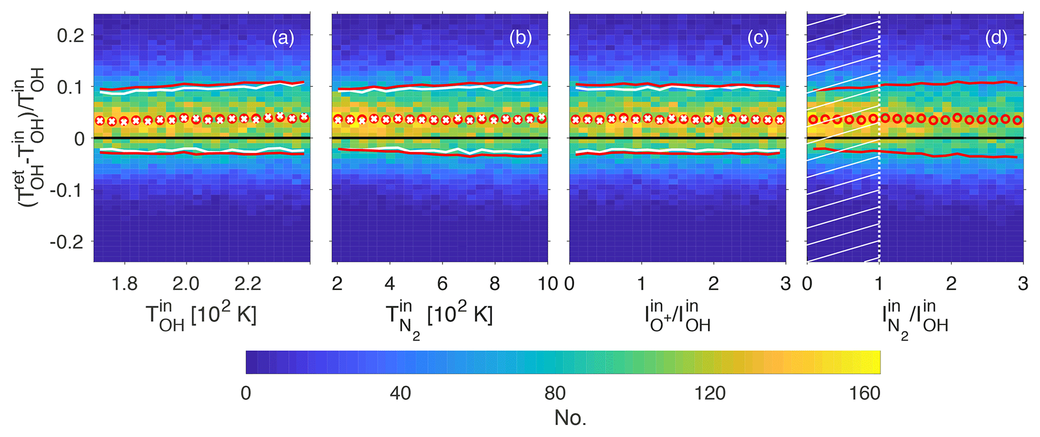
Figure 9 2-D histograms of parameter retrieval tests showing the fractional error on OH temperature retrieval when the synthetic spectra are constructed using a different source for the transition probabilities of the OH lines (Langhoff et al., 1986) than used in the retrieval process (Mies, 1974). Red circles indicate mean values and red lines are 1 standard deviation on either side of the mean. The white crosses and white solid lines in panels (a, b, c) represent mean values and 1 standard deviation on either side of the mean, respectively, but only including spectra for the N₂ intensity within the hatched area shown in panel (d).

5.6 Noise considerations

We have assumed that the main noise present in HiTIES spectra is shot noise, neglecting read-out and thermal sources of noise. HiTIES is equipped with an EMCCD chip, meaning that there is no read-out noise. Thermal noise should be low since the instrument is cooled to −80 ^∘C; however, we have run additional simulations to estimate an upper limit on noise of thermal origin. To model thermal noise, we take a Gaussian distribution with a standard deviation of 62 R nm⁻¹, corresponding to the mean absolute value of the residuals of the spectral fit shown in Fig. 2b. We then run the Monte Carlo simulation including both shot and thermal noise. The results are qualitatively identical to those presented in the previous sections, with uncertainty values increased by about 1 %. This is an upper limit since it assumes that the level of the residuals is caused by thermal noise alone.

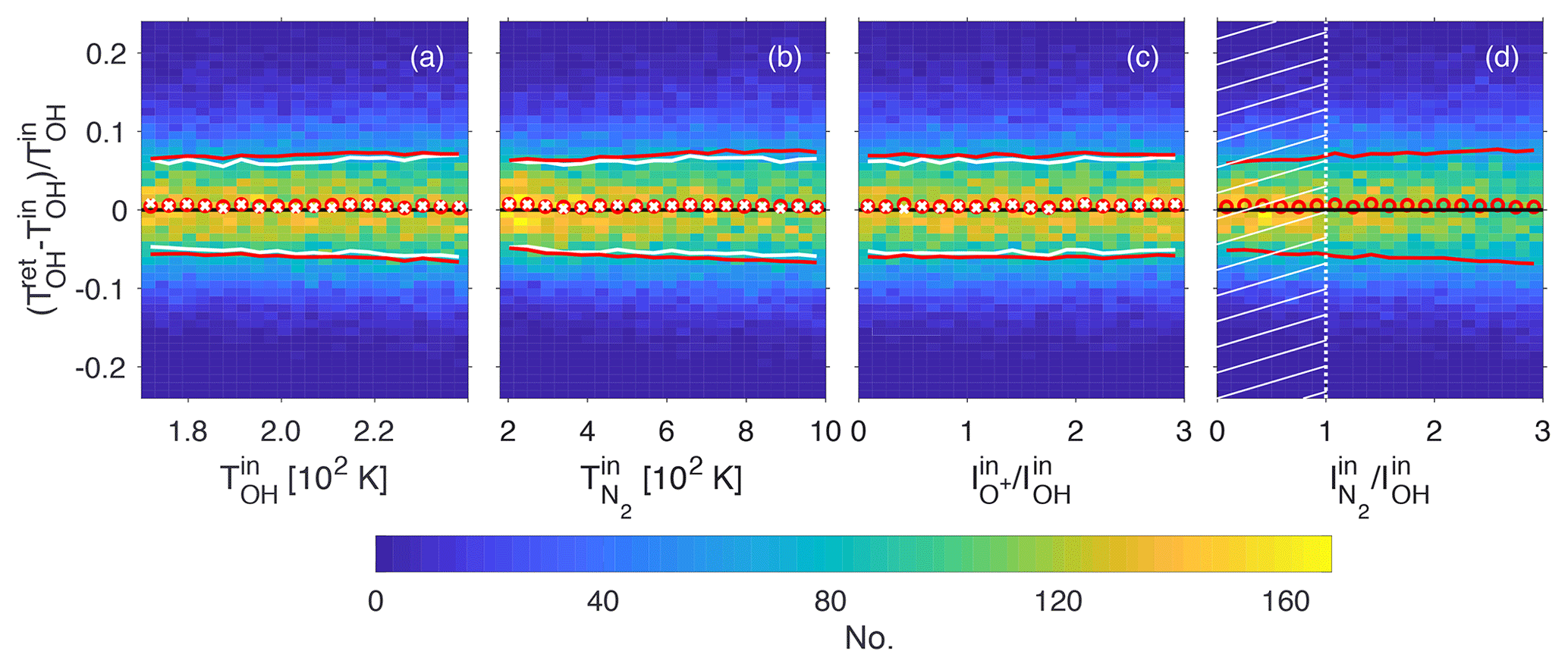
Figure 10 2-D histograms of parameter retrieval tests showing the fractional error on OH temperature retrieval when the synthetic spectra are constructed using a different source for the energy levels of excited OH (Coxon and Foster, 1982) than used in the retrieval process (Krassovsky et al., 1962). Red circles indicate mean values and red lines are 1 standard deviation on either side of the mean. The white crosses and white solid lines in panels (a, b, c) represent mean values and 1 standard deviation on either side of the mean, respectively, but only including spectra for the N₂ intensity within the hatched area shown in panel (d).

6 Assessment of uncertainties on OH quantum numbers

The OH temperature measurements depend on possessing correct values of transition probabilities and energy terms. In particular, past studies have shown large differences in OH temperatures derived using different sources for the transition probabilities (Phillips et al., 2004). To assess this effect on our retrieval process, we have constructed 10 000 synthetic spectra in the same manner as described in Sect. 5, except that they are constructed using transition probabilities from Langhoff et al. (1986), whereas the retrieval process assumes transition probabilities from Mies (1974). The results of this Monte Carlo simulation are shown in Fig. 9, in which the same parameters are plotted as in the top row of Fig. 6; namely, the fractional error on the OH temperature is plotted against the OH temperature (panel a), the N₂ temperature (panel b), the O⁺ intensity (panel c), and the N₂ intensity (panel d). The 2-D histograms in Fig. 9 are very similar to those in the top row of Fig. 6, in which the transition probabilities used both in constructing the synthetic spectra and in the retrieval process are from Mies (1974). The only difference is an offset of about 3 % to 4 %, corresponding to a difference in temperature of 6 to 8 K, assuming an OH temperature of around 200 K.

We take the same approach to ascertain the effect on OH temperatures of different sources for the OH energy levels. The fractional errors on the retrieval of T_OH are plotted in Fig. 10 by constructing synthetic spectra with energy terms from Coxon and Foster (1982) and assuming Krassovsky et al. (1962) values in the retrieval process. The mean values also show an offset from the 0 error line, but much smaller than for different transition probabilities, of about 0.5 % to 1 %, equivalent to 1 to 2 K at 200 K.

7 Conclusions

We have developed a new spectral fitting method that allows us to extract the intensity of simultaneous emissions in HiTIES spectra. These emissions – OH airglow, auroral O⁺, and N₂ – originate from different atmospheric layers and their properties inform us of the state of the upper polar atmosphere. In particular, combining our spectral fitting method with a temperature retrieval process allows us to estimate neutral temperatures at different altitudes and the atmospheric column density of water vapour. In this paper, using a Monte Carlo simulation to retrieve the known parameters of synthetic spectra, we have shown the domains over which our spectral fitting and temperature retrieval processes are successful.

The Monte Carlo simulation shows that we can correctly retrieve OH temperatures, as long as any N₂ emission is not too bright. Indeed, we find that the distribution of fractional errors on T_OH has a standard deviation of less than 6 % when the maximum intensity of the N₂ spectrum is less than the peak intensity of the strongest OH emission line seen in HiTIES, OH(8-3) P₁(3). This uncertainty corresponds to about 12 K on an OH temperature of 200 K, obtained from a single spectrum typically integrated over 2 min of observing time. Since OH emission is present in almost all of our data, we can improve the errors on T_OH by temporally averaging multiple observations. Thus, combining 15 consecutive 2 min measurements would reduce the absolute uncertainty from 12 to 3.1 K.

We have also evaluated the magnitude of errors on T_OH that occurs from uncertainties in the OH transition probabilities. The offset measured between temperatures obtained using transition probabilities from Mies (1974) and Langhoff et al. (1986) is about 4 % on average (roughly 8 K), reinforcing the fact that any comparisons between different OH temperature datasets must take this into account.

When there is sufficient N₂ emission present, we can successfully determine the N₂ temperature. The standard deviation of the distribution of fractional errors on $T_{{\mathrm{N}}_{\mathrm{2}}}$ is between 3 % and 5 % when the maximum intensity of the N₂ spectrum is greater than 3.7 times the background level. In the spectral fitting procedure and the Monte Carlo simulations performed in this study, we have assumed that all of the N₂ emission in the HiTIES spectrum is produced at a single temperature. This is not necessarily the case, especially if the N₂ layer is extended in altitude. Therefore, in future we intend to modify our spectral fitting method to take into account the possible presence of N₂ emission at different temperatures in a single spectrum.

Whiter et al. (2014) showed that the ratio of the two O⁺ doublets observed by HiTIES at 732 and 733 nm can be used as a measure of the neutral temperature in the F-region ionosphere. We can determine this ratio, $R_{{\mathrm{O}}^{+}}$, with a distribution of fractional errors of less than 5 % when the peak of the 732 nm O⁺ doublet is greater than 6 times the background emission.

As a by-product of the spectral fitting method, we have been able to estimate the amount of water vapour in the column of atmosphere above the HiTIES instrument: the precipitable water vapour or PWV. When OH lines are present in our data, which is almost at all times that the instrument is running, we can obtain high-cadence (at least every 10 min) measurements of the PWV.

In a number of follow-up studies, we will make use of the spectral fitting and temperature retrieval methods demonstrated here to explore trends in upper atmospheric neutral temperatures in the HiTIES dataset. As a first step, we shall compare OH(8-3) temperatures measured by HiTIES with OH(6-2) temperatures from the Silverbullet instrument operated by the University Centre in Svalbard (UNIS) (Holmen et al., 2014; Sigernes et al., 2003), also located at the Kjell Henriksen Observatory, and with OH temperatures derived from the SABER instrument onboard the TIMED satellite.