In-orbit results of the Coupled Dark State Magnetometer aboard the China Seismo-Electromagnetic Satellite

The China Seismo-Electromagnetic Satellite (CSES) was launched in February 2018 into a polar, sun-synchronous, low Earth orbit. It provides the first demonstration of the Coupled Dark State Magnetometer (CDSM) measurement principle in space. The CDSM is an optical scalar magnetometer based on the coherent population trapping (CPT) effect and measures the scalar field with the lowest absolute error aboard CSES. Therefore, it serves as the reference instrument for the measurements done by the fluxgate sensors within the High Precision Magnetometer instrument package.

In this paper several correction steps are discussed in order to improve the accuracy of the CDSM data. This includes the extraction of valid 1 Hz data, the application of the sensor heading characteristic, the handling of discontinuities, which occur when switching between the CPT resonance superpositions, and the removal of fluxgate and satellite interferences.

The in-orbit performance is compared to the Absolute Scalar Magnetometer aboard the Swarm satellite Bravo via the CHAOS magnetic field model. Additionally, an uncertainty of the magnetic field measurement is derived from unexpected parametric changes of the CDSM in orbit in combination with performance measurements on the ground.

1 Introduction

The China Seismo-Electromagnetic Satellite (CSES), also known as Zhangheng-1, investigates natural electromagnetic phenomena and possible applications for earthquake monitoring from space (Shen et al., 2018). CSES was launched in February 2018 into a polar, sun-synchronous, low Earth orbit with an inclination of approximately 97^∘ and a period of approximately 95 min. The High Precision Magnetometer (HPM) instrument package (Cheng et al., 2018) consists of two fluxgate magnetometers (FGMs) in a gradiometer configuration and the Coupled Dark State Magnetometer (CDSM). The CDSM measures the magnetic field strength with the lowest absolute error of the instruments aboard CSES and serves as the reference instrument for the measurements done by the fluxgate sensors. The suitability of the CDSM for the in-flight calibration of the fluxgate magnetometers is discussed in Zhou et al. (2019).

The CDSM is an optical scalar magnetometer based on a quantum interference effect called coherent population trapping (CPT) (Arimondo, 1996; Wynands and Nagel, 1999), which inherently enables omnidirectional measurements (Lammegger, 2008; Pollinger et al., 2012) and an all-optical sensor design without double cell units, excitation coils or active electronics parts (Pollinger et al., 2018).

Figure 1 Laser excitation scheme within the D₁-line hyperfine structure of ⁸⁷Rb.

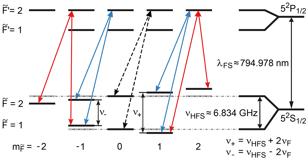
The instrument simultaneously probes several CPT resonances which are established within the D₁-line hyperfine structure (HFS) of ⁸⁷Rb shown in Fig. 1. Here, the total angular momentum quantum numbers and the magnetic quantum numbers of the 5²S_1∕2 ground states are denoted by $\stackrel{\mathrm{̃}}{F}$ and correspondingly by $m_{\stackrel{\mathrm{̃}}{F}}$, while for the 5²P_1∕2 excited states the labels are primed. The wavelength λ_FS corresponds to the fine structure transition ${\mathrm{5}}^{\mathrm{2}}{\mathrm{S}}_{\mathrm{1}/\mathrm{2}}\to {\mathrm{5}}^{\mathrm{2}}{\mathrm{P}}_{\mathrm{1}/\mathrm{2}}$. The HFS ground state splitting frequency is denoted by ν_HFS. The energy shift introduced by the magnetic field is expressed by ν_F. For the excitation of each CPT resonance, a Λ-shaped excitation scheme is prepared in the HFS, which consists of three energy levels interacting with two light fields indicated by the arrowed lines in Fig. 1.

In order to create the necessary light fields, a vertical-cavity surface-emitting laser (VCSEL) diode (vacuum wavelength ${\mathit{\lambda }}_{\mathrm{Laser}}={\mathit{\lambda }}_{\mathrm{FS}}\approx \mathrm{794.978}$ nm) is frequency-modulated (FM) by a microwave oscillator signal ($f_{\mathrm{MW}}=\mathrm{1}/\mathrm{2}\cdot {\mathit{\nu }}_{\mathrm{HFS}}$ ≈3.417 GHz). The CPT resonance n=0 is excited by the two light fields denoted by the black dashed arrowed lines in Fig. 1 and occurs under certain conditions when the frequency difference of both first-order sidebands of this FM spectrum fits the energy difference of the 5²S_1∕2 ground states $\stackrel{\mathrm{̃}}{F}=\mathrm{1}$, $m_{\stackrel{\mathrm{̃}}{F}}=\mathrm{0}$ and $\stackrel{\mathrm{̃}}{F}=\mathrm{2}$, $m_{\stackrel{\mathrm{̃}}{F}}=\mathrm{0}$. This resonance is used to adjust the microwave oscillator frequency to changes in ν_HFS and to compensate for a temperature-dependent drift of the electronics.

An additional modulation of the microwave oscillator signal probes the first-order Zeeman splitting of HFS ground states via the superposition of the CPT resonances $n=+\mathrm{2}$ and −2 or $n=+\mathrm{3}$ and −3, which are indicated by the red and blue arrowed lines in Fig. 1, respectively. The differential probing of the magnetic-field-induced energy shifts, with one of the two CPT resonance pairs, cancels or at least mitigates the influence of sensor temperature variations on the magnetic field measurement (Lammegger, 2008; Pollinger et al., 2018).

The instrument consists of a mixed signal electronics board and a laser unit, which are mounted in an instrument box inside the spacecraft body, as well as a sensor unit which is located outside the satellite at the tip of a boom. Additionally, the instrument box and the sensor unit are connected with two optical fibres and two twisted pair cables to guide the light field to and from the sensor unit and to control the sensor temperature (Pollinger et al., 2018).

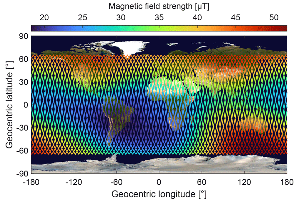
Figure 2 Magnetic field strength measured by the CDSM within ±65^∘ of geocentric latitude for the reoccurrence period of 5 d. Credit for the background image: Reto Stöckli, NASA Earth Observatory.

The CDSM development started in 2007, and the instrument measured the magnetic field in space for the first time in March 2018 aboard CSES. As far as we know, this was also the first time a magnetometer based on the CPT effect was launched into space. Since then, the instrument has been operational and orbited Earth more than 12 000 times until April 2020. The main scientific objective of the CSES mission is within ±65^∘ of geocentric latitude, and most of the attitude control activities are moved outside this area to the polar regions (Shen et al., 2018; Zhou et al., 2019). The data transfer is separated into a 1 Hz channel for all latitudes and a channel with higher instrument update rates for the area within ±65^∘ of geocentric latitude. The 1 Hz channel is mainly used for housekeeping purposes and is not accessible for the CDSM team. Figure 2 shows the magnetic field strength measured by the CDSM along the CSES orbit tracks within ±65^∘ of geocentric latitude for the 5 d reoccurrence period of 3–8 January 2019.

Figure 3 Minimum and maximum optical power detected at the photodiode during individual orbit segments.

All available housekeeping data are within the nominal operational limits throughout the elapsed mission time. As an example, the minimum and maximum optical power detected at the photodiode on the electronics board are shown for individual orbit segments in Fig. 3. The light is generated in the laser unit and guided through two optical fibres to and from the sensor unit where it interacts with the rubidium atoms and derives information on the surrounding magnetic field. The optical power received at the photodiode is an indicator for the health of the VCSEL diode (Ellmeier et al., 2018), the fibres, the optical components in the sensor and the photodiode. The graph in Fig. 3 shows gaps since not all data were made available to the CDSM team or the satellite was in safe mode in which the scientific instruments were switched off. The optical power varies due to the design of the CDSM (Pollinger et al., 2018). It is assumed that the different exposures to sunlight cause thermal stress in the multimode outbound fibre, which results in a variation of the polarization state at the sensor input. Behind the polarizer in the sensor unit a defined linear polarization state is re-established with the consequence that the optical power varies. No trend is visible in Fig. 3, and the minimum optical power was above the operational limit of 5 µW throughout the available data for the elapsed mission time.

Each orbit is divided into two orbit segments, and data are stored separately in Hierarchical Data Format 5 (HDF5) files for each orbit segment. Dayside and nightside orbit segments are marked with the suffixes 0 and 1, respectively. For example, 44270 is the identifier for the daytime ascending segment of orbit 4427.

2 Correction of in-orbit data

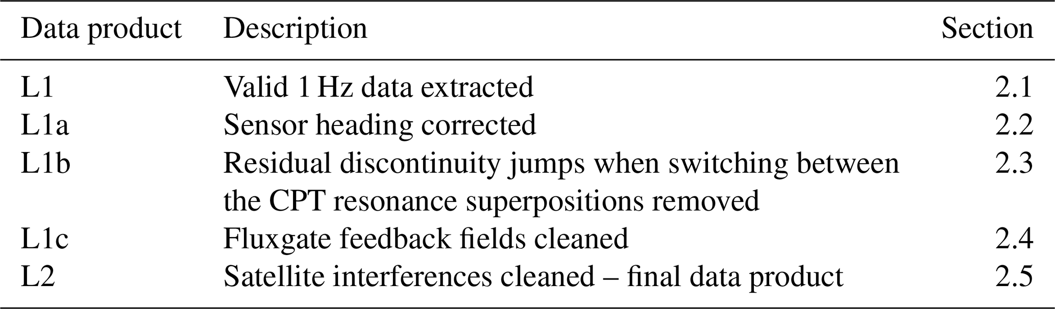
Several correction steps are required in order to improve the accuracy of the CDSM data. This includes the extraction of valid 1 Hz data, the application of the sensor heading characteristic, the handling of discontinuities, which occur when switching between the CPT resonance superpositions, and the removal of fluxgate and satellite interferences. Table 1 lists these steps and introduces data product labels. L1a, L1b and L1c are not official data products.

Table 1 CDSM data products and correction steps.

2.1 Extraction of valid 1 Hz data

The raw data rate of the CDSM is 30 Hz. However, every second is divided in three subsequent parts: the first third of each second is reserved for the sensor heating, the second third of each second for adjusting the microwave oscillator to track the CPT resonance n=0 and the last third of each second for the actual magnetic field measurement by tracking the CPT resonance superposition $n=\pm \mathrm{2}$ or $n=\pm \mathrm{3}$.

The CPT resonances n=0, $n=+\mathrm{2}$, $n=-\mathrm{2}$, $n=+\mathrm{3}$ and $n=-\mathrm{3}$ depend differently on the magnetic strength in second order (57.515 kHz mT⁻² for n=0, 43.136 kHz mT⁻² for $n=\pm \mathrm{2}$ and 21.568 kHz mT⁻² for $n=\pm \mathrm{3}$). As a consequence, the CPT resonance n=0 is not in the centre of the single CPT resonances $n=+\mathrm{2}$ and $n=-\mathrm{2}$ or $n=+\mathrm{3}$ and $n=-\mathrm{3}$ used for magnetic field measurement. Thus, the modulation of the microwave oscillator signal would not probe the single CPT resonances $n=+\mathrm{2}$ and −2 or $n=+\mathrm{3}$ and −3 at the same time. With the fact that individual single CPT resonances can have different line shapes, this might cause a deviation of the magnetic field measurement (Pollinger et al., 2018). This cannot be ignored for CSES where the magnetic field strength is between 18 and 52 µT.

Therefore, during the last third of every second, the microwave oscillator control loop for tracking the CPT resonance n=0 is paused and the latest microwave oscillator control value is corrected by an offset in order to re-centre the microwave oscillator signal with respect to the single CPT resonances $n=+\mathrm{2}$ and $n=-\mathrm{2}$ or $n=+\mathrm{3}$ and $n=-\mathrm{3}$. Details are discussed in Sect. 3.2 and Pollinger et al. (2018).

An additional control loop tracks the CPT resonance superposition $n=\pm \mathrm{2}$ or $n=\pm \mathrm{3}$ and continuously delivers magnetic field values. However, only the last seven samples of every second are considered to be unaffected by the influence of the sensor heater current, by deviations due to the second-order magnetic field dependence or by those linked to transients in the magnetic field strength read-out. Every second the mean value of these last seven samples is tagged with the time stamp of the fourth of the last seven samples. The mean values serve as 1 Hz raw data for the CDSM instrument.

2.2 Application of sensor heading characteristic

The CDSM read-out has a deviation of the actual magnetic field strength, which depends on the angle between the light propagation direction through the sensor and the magnetic field vector (from here on called the sensor angle). This heading is characteristic for the flight model and was determined during performance tests in the assembled HPM configuration at the Fragment Mountain Weak Magnetic Laboratory of the National Institute of Metrology in China (Pollinger et al., 2018). The 1 Hz raw data are corrected by this heading characteristic according to the magnetic field direction derived from the HPM fluxgate data.

As an example Fig. 4a shows the magnetic field strength measured by the CDSM during orbit segment 44270. In order to show details on the correction process, the magnetic field strength calculated with CHAOS-6 (Finlay et al., 2016; Olsen et al., 2006), a geomagnetic Earth field model derived from the Swarm, CHAMP, Ørsted and SAC-C satellites as well as ground observatory data, was subtracted.

Figure 4b displays sign-changed heading measurements derived from Pollinger et al. (2018) and the angular-dependent heading correction applied for the orbit segment 44270. The heading correction pattern is not continuous over an orbit segment. The CDSM uses one of the two CPT resonance superpositions $n=\pm \mathrm{2}$ or $n=\pm \mathrm{3}$ to enable omnidirectional magnetic field measurements (Pollinger et al., 2012). The selection depends on the sensor angle. For angles between approximately 0 and 60^∘ as well as 120 and 180^∘ the signal amplitude of the CPT resonance superposition $n=\pm \mathrm{2}$ is large enough to be used, while for angles between approximately 60 and 120^∘ only the superposition $n=\pm \mathrm{3}$ is applicable. In flight, the CDSM gets HPM fluxgate data to switch between these two resonance superpositions at 60 and 120^∘ with an intended hysteresis of approximately 2^∘. The actual switching angles vary with ±1^∘ due to a basic on-board fluxgate correction. For the descending orbit segment 44270 shown in Fig. 4a, the sensor angle changed from approximately 165 to 27^∘. The instrument switched from the CPT resonance superposition $n=\pm \mathrm{2}$ to $n=\pm \mathrm{3}$ at approximately 117^∘ and from the CPT resonance superposition $n=\pm \mathrm{3}$ to $n=\pm \mathrm{2}$ at approximately 58^∘. The heading correction for the CPT resonance superposition $n=\pm \mathrm{2}$ was refined compared to the linear fit in Pollinger et al. (2018) to better represent the characteristic seen during various measurements on the ground. Now, measurements with the CPT resonance superposition $n=\pm \mathrm{2}$ are corrected with a second-order polynomial fit. The origin of the heading characteristic is still under investigation.

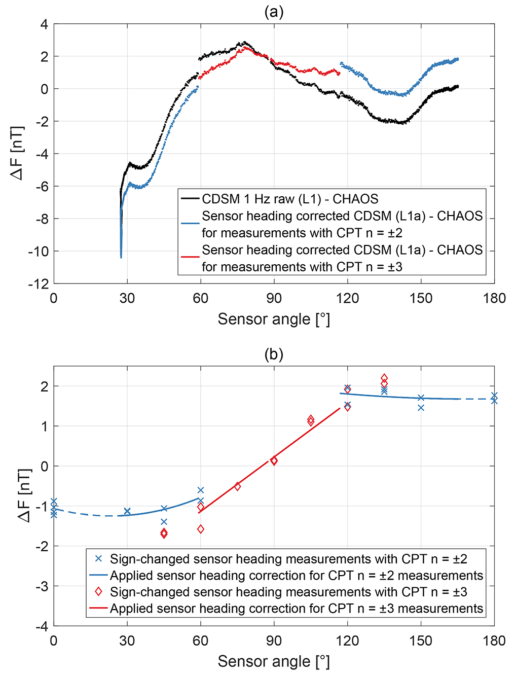
Figure 4 Example for applying the sensor heading characteristic and the corresponding correction pattern derived from measurements on the ground.

2.3 Removal of residual discontinuity jumps when switching CPT resonance superpositions

After the sensor heading correction, the magnetic field values are not continuous when the resonance superpositions $n=\pm \mathrm{2}$ and $n=\pm \mathrm{3}$ are switched. For example, Fig. 5a shows the magnetic field strength measured by the CDSM during the orbit segment 44270 with the CHAOS-6 calculation subtracted. When switching from the CPT resonance superposition $n=\pm \mathrm{2}$ to $n=\pm \mathrm{3}$ a jump of the magnetic field strength of approximately −0.71 nT is observable in the CDSM read-out, while for the change from CPT resonance superposition $n=\pm \mathrm{3}$ to $n=\pm \mathrm{2}$ the step is approximately −0.66 nT. These discontinuity jumps vary with each orbit segment and are further discussed in Sect. 3.2.

In order to avoid a misinterpretation by the scientific user, the discontinuity jumps are removed individually for each orbit segment by adjusting the magnetic field data derived with the CPT resonance superposition $n=\pm \mathrm{3}$ to measurements with the CPT resonance superposition $n=\pm \mathrm{2}$.

When switching from CPT resonance superposition $n=\pm \mathrm{2}$ to $n=\pm \mathrm{3}$ the signal amplitude of the CPT resonance n=0 is also small and the microwave oscillator control loop is paused (Pollinger et al., 2018). For the subsequent measurements with the CPT resonance superposition $n=\pm \mathrm{3}$ the last microwave oscillator control value is re-centred as discussed in Sect. 2.1. When switching from the CPT resonance superposition $n=\pm \mathrm{3}$ to $n=\pm \mathrm{2}$ the signal of the CPT resonance n=0 is large enough to re-activate the control loop. Consequently, for measurements with the CPT resonance superposition $n=\pm \mathrm{2}$ the microwave oscillator control loop is active. Then it can compensate for a possible temperature drift of the electronics and can follow a change in the HFS ground state splitting due to e.g. a sensor temperature drift.

For each orbit segment the two discontinuity jumps at the resonance transitions are used to calculate a linear ramp. The ramp is added to the magnetic field strength measured with CPT resonance superposition $n=\pm \mathrm{3}$. As an example this correction pattern is shown for the orbit segment 44270 in Fig. 5b.

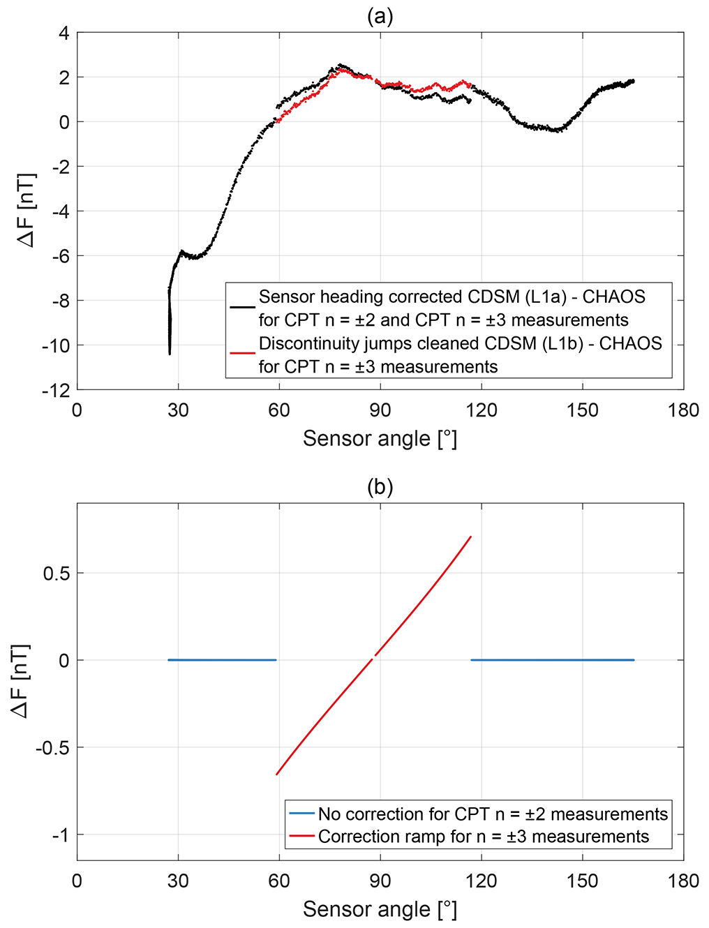
Figure 5 Example for removing residual discontinuity jumps, which occur when switching CPT resonance superpositions, and the corresponding correction pattern.

2.4 Removal of fluxgate interferences

The HPM sensor configuration consists of the CDSM sensor mounted at the tip of a 4.7 m long boom, while the FGM 2 and FGM 1 sensors are located 0.367 and 0.767 m inwardly.

Fluxgates are inherently zero field detection devices with which an artificial magnetic field is applied to cancel the environmental magnetic field in the sensor (Auster, 2008). For CSES this field can significantly influence the magnetic field measurement of the other sensors. The cross interferences were characterized with the sensors mounted on a dummy boom in a µ-metal chamber (Zhou et al., 2018). The FGM 1 and FGM 2 sensors were located at the correct distances and orientation with respect to the CDSM position. The CDSM was replaced by a third fluxgate sensor for this test. The influence of the FGM 2 feedback field F_FG 2 at the CDSM sensor position is

$$\begin{array}{}\text{(1)}& \begin{array}{rl}& \left[\begin{array}{c}{F}_{\mathrm{FG}\mathrm{2},x_{\mathrm{FG}\mathrm{2}}}\\ F_{\mathrm{FG}\mathrm{2},y_{\mathrm{FG}\mathrm{2}}}\\ F_{\mathrm{FG}\mathrm{2},z_{\mathrm{FG}\mathrm{2}}}\end{array}\right]=\mathbf{I}\left[\begin{array}{c}{F}_{x_{\mathrm{FG}\mathrm{2}}}\\ F_{y_{\mathrm{FG}\mathrm{2}}}\\ F_{z_{\mathrm{FG}\mathrm{2}}}\end{array}\right]\\ & ={\mathrm{10}}^{-\mathrm{5}}\left[\begin{array}{ccc}\mathrm{5.34}& \mathrm{1.97}& \mathrm{0.67}\\ \mathrm{1.33}& -\mathrm{7.82}& \mathrm{0.00}\\ \mathrm{0.00}& \mathrm{1.90}& \mathrm{2.76}\end{array}\right]\left[\begin{array}{c}{F}_{x_{\mathrm{FG}\mathrm{2}}}\\ F_{y_{\mathrm{FG}\mathrm{2}}}\\ F_{z_{\mathrm{FG}\mathrm{2}}}\end{array}\right],\end{array}\end{array}$$

where I is the matrix characteristic of the FGM 2 feedback field influence, which depends on the Earth's magnetic field vector F. The FGM 2 sensor coordinates x_FG 2, y_FG 2, and z_FG 2 correspond to the satellite coordinates y_sat, z_sat and x_sat, respectively, where x_sat is approximately the flight direction and z_sat points approximately to the centre of Earth. The matrix characteristic of the FGM 1 feedback field influence is not available from ground tests. Nevertheless, with the same sensor design, orientation and given location, the influence of the FGM 1 feedback field F_FG 1 at the CDSM sensor position can be estimated as

$$\begin{array}{}\text{(2)}& \left[\begin{array}{c}{F}_{\mathrm{FG}\mathrm{1},x_{\mathrm{FG}\mathrm{2}}}\\ F_{\mathrm{FG}\mathrm{1},y_{\mathrm{FG}\mathrm{2}}}\\ F_{\mathrm{FG}\mathrm{1},z_{\mathrm{FG}\mathrm{2}}}\end{array}\right]\approx \mathrm{0.11}\left[\begin{array}{c}{F}_{\mathrm{FG}\mathrm{2},x_{\mathrm{FG}\mathrm{2}}}\\ F_{\mathrm{FG}\mathrm{2},y_{\mathrm{FG}\mathrm{2}}}\\ F_{\mathrm{FG}\mathrm{2},z_{\mathrm{FG}\mathrm{2}}}\end{array}\right],\end{array}$$

where F_FG 2 is the influence of the FGM 2 feedback field at the CDSM sensor position and x_FG 2, y_FG 2 and z_FG 2 are the FGM 2 sensor coordinates. The CDSM scalar measurement is transformed into a vector as a function of F derived by FGM 2 and is corrected by F_FG 1 and F_FG 2. In orbit the impact of the fluxgate sensors is up to 4.4 nT at the CDSM position, and it depends on the magnetic field direction and strength. As an example the influence of the fluxgates during orbit segment 44270 is shown in Fig. 6.

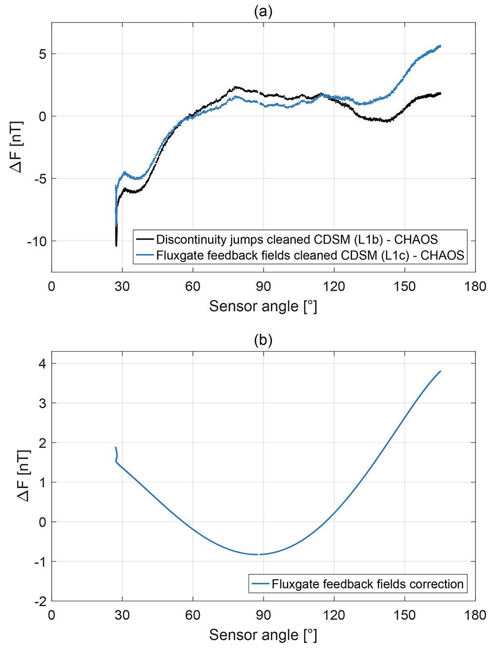
Figure 6 Example for the influence of the fluxgate feedback fields and the corresponding correction pattern.

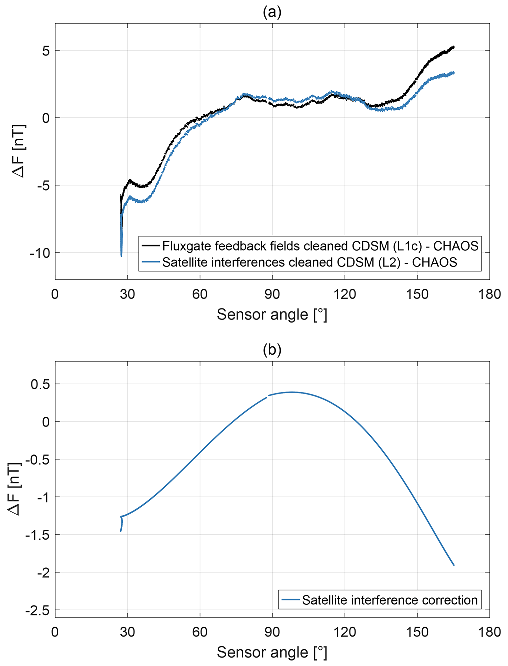
2.5 Removal of satellite interferences

Although there was a magnetic cleanliness programme carried out by the satellite developer, some magnetic disturbances remain visible to the magnetometers. In order to be able to remove these interferences from the scientific data the whole satellite was installed in a coil system and different operation modes were magnetically measured. The influence of the satellite F_sat at the CDSM sensor position was published in Xiao et al. (2018) as

$$\begin{array}{}\text{(3)}& \begin{array}{rl}& \left[\begin{array}{c}{F}_{\mathrm{sat},x_{\mathrm{sat}}}\\ F_{\mathrm{sat},y_{\mathrm{sat}}}\\ F_{\mathrm{sat},z_{\mathrm{sat}}}\end{array}\right]=\mathbf{A}\left[\begin{array}{c}{F}_{x_{\mathrm{sat}}}\\ F_{y_{\mathrm{sat}}}\\ F_{z_{\mathrm{sat}}}\end{array}\right]+{\mathit{F}}_{\mathrm{0}}+\mathbf{C}\left[\begin{array}{c}{M}_{x_{\mathrm{sat}}}\\ M_{y_{\mathrm{sat}}}\\ M_{z_{\mathrm{sat}}}\end{array}\right]\\ & ={\mathrm{10}}^{-\mathrm{5}}\left[\begin{array}{ccc}-\mathrm{1.108}& \mathrm{0.025}& \mathrm{0.725}\\ -\mathrm{0.350}& -\mathrm{2.808}& -\mathrm{1.100}\\ \mathrm{1.225}& -\mathrm{1.158}& \mathrm{4.658}\end{array}\right]\left[\begin{array}{c}{F}_{x_{\mathrm{sat}}}\\ F_{y_{\mathrm{sat}}}\\ F_{z_{\mathrm{sat}}}\end{array}\right]\\ & +\left[\begin{array}{c}-\mathrm{0.16}\\ -\mathrm{0.26}\\ \mathrm{0.29}\end{array}\right]+\left[\begin{array}{ccc}\mathrm{0.20}& \mathrm{0.01}& \mathrm{0.00}\\ \mathrm{0.03}& \mathrm{0.56}& -\mathrm{0.01}\\ -\mathrm{0.08}& \mathrm{0.07}& -\mathrm{0.47}\end{array}\right]\left[\begin{array}{c}{M}_{x_{\mathrm{sat}}}\\ M_{y_{\mathrm{sat}}}\\ M_{z_{\mathrm{sat}}}\end{array}\right],\end{array}\end{array}$$

where A is the matrix characteristic of the soft magnetic influences, which depends on the Earth's magnetic field vector F, F₀ is the remanence of hard magnetic materials and C is the matrix characteristic of the magnetorquer influence which depends on the torque states M. The coordinates x_sat, y_sat and z_sat correspond to the satellite where x_sat is approximately the flight direction and z_sat points approximately to the centre of Earth. The CDSM scalar measurement is transformed into a vector as a function of F derived by FGM 2 and is corrected by F_sat. As an example, the influence of the satellite during the orbit segment 44270 is shown in Fig. 7.

Figure 7 Example of the satellite interferences and the corresponding correction pattern.

3 In-orbit performance

The CDSM is the magnetometer with the lowest absolute error aboard CSES. Therefore, the in-orbit performance of the CDSM can solely be obtained by comparing its measurements to magnetic field models, measurements from other satellite missions or through a study of the integrity of its own data.

3.1 Comparison to CHAOS model and Swarm data

The CDSM data were compared to the CHAOS-6 model (Finlay et al., 2016; Olsen et al., 2006). The CHAOS model is optimized for the nightside, which means that the CHAOS coefficients are determined in such a way as to minimize the difference between the CHAOS model and Earth's magnetic field on the nightside. These residuals are dominated by a magnetospheric ring-current contribution, which is not included in the CHAOS model and which shows a minimum scatter at around ±35^∘ of dipole latitude. Therefore, the mean values and standard deviations, which are calculated for the dipole latitude ranges of −40 to −30^∘ (southern evaluation interval) and 30 to 40^∘ (northern evaluation interval), are an indicator for the magnetometer's data quality. Additionally, only data with a Kp index smaller than 1 have been selected for this evaluation. The Kp index quantifies disturbances in the horizontal component of the Earth's magnetic field (Bartels et al., 1939).

With an ascending node at approximately 02:00 and an inclination of approximately 97^∘, the actual local time of CSES nightside orbit segments is between approximately 01:00 and 03:00. Swarm is a three-satellite low Earth orbit mission of the European Space Agency launched in 2013 to study the Earth's magnetic field. Each satellite contains an Absolute Scalar Magnetometer (ASM) as a reference instrument. The Swarm satellite Bravo has an inclination of approximately 88^∘, and the ascending and descending nodes drift. Between 15 and 30 November 2018 the ascending nodes of Swarm Bravo were between 02:38 and 01:19 and 48–42 min after the ascending nodes of CSES. The local time ranges overlapped for the Swarm and CSES nightside orbit segments. Data for this time interval have been selected for the comparison. The altitude of the Swarm satellite Bravo was between 501 and 518 km, while CSES orbited at 500–511 km during the selected time interval.

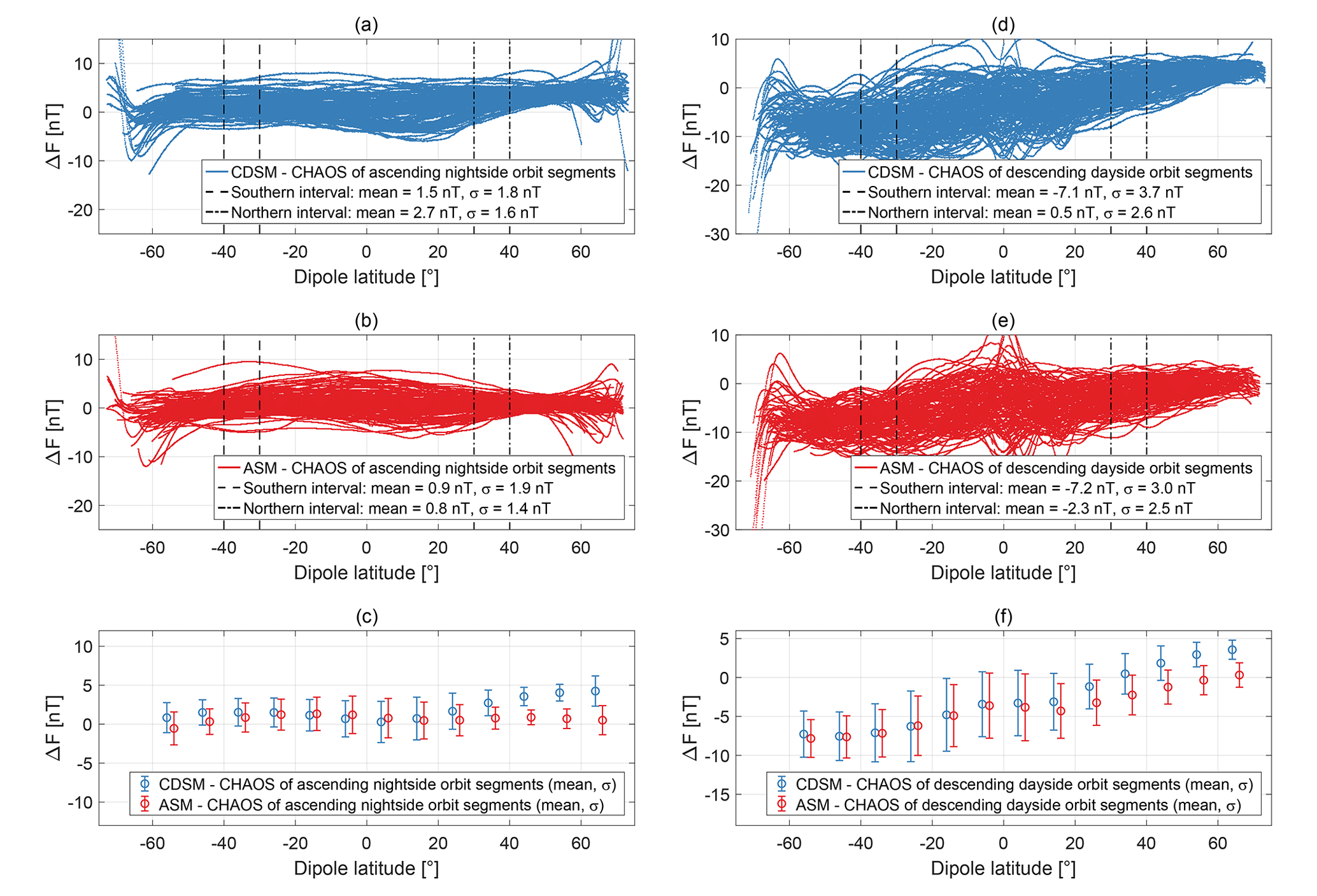
Figure 8 Magnetic field strength measured by CDSM compared to Swarm Bravo ASM via the CHAOS-6 Earth field model for nightside and dayside orbit segments.

Figure 8a shows the difference between CDSM measurements and the CHAOS-6 model for the 135 selected night-time orbit segments, while Fig. 8b displays the equivalent analysis for the ASM aboard Swarm satellite Bravo. The mean values $\stackrel{\mathrm{‾}}{\mathrm{\Delta }F}$ and standard deviations σ of the differences to the CHAOS model were calculated with a 10^∘ resolution of the dipole latitude. These values are shown as error bars for each individual instrument in Fig. 8c.

The mean values of both instrument deviations are consistent in the magnetic dipole latitude range of −40 to −30^∘ ($\stackrel{\mathrm{‾}}{\mathrm{\Delta }F}=\mathrm{1.5}$ nT, σ=1.8 nT for CDSM and $\stackrel{\mathrm{‾}}{\mathrm{\Delta }F}=\mathrm{0.9}$ nT, σ=1.9 nT for ASM). One can see that the 1σ error bars of both instruments match in size and mean values widely but start to separate at dipole latitudes greater than 20^∘. For the dipole latitude range of 30 to 40^∘ the mean values of both instruments differ by 1.9 nT ($\stackrel{\mathrm{‾}}{\mathrm{\Delta }F}=\mathrm{2.7}$ nT for CDSM and $\stackrel{\mathrm{‾}}{\mathrm{\Delta }F}=\mathrm{0.8}$ nT for ASM). Similar differences between the CDSM and the ASM mean values can also be observed for dayside orbit segments in Fig. 8d, e and f.

3.2 Discussion of data integrity

For the analysis in this section data from 9387 of 13 058 possible orbit segments between 16 November 2018 and 19 January 2020 were available. As already discussed in Sect. 2.3 the magnetic field values are not continuous when the resonance superpositions $n=\pm \mathrm{2}$ and $n=\pm \mathrm{3}$ are switched. Histograms of these discontinuity jumps are presented in Sect. 3.2.1. All available instrument parameters, especially the microwave oscillator frequency controller adjustment, are investigated in detail. The sensitivity of the magnetic field measurement as a function of a microwave oscillator frequency detuning is derived in Sect. 3.2.2. The variations of housekeeping parameters, such as the optical power received at the photodiode as well as the sensor and printed circuit board (PCB) temperatures, are discussed in Sect. 3.3.3, 3.3.4 and 3.3.5, respectively. In Sect. 3.3.6, an angular-dependent adjustment of the microwave oscillator frequency is presented, which could be observed for measurements with the CPT resonance superposition $n=\pm \mathrm{2}$ during ground tests with the flight model. Some influences are understood and can be subtracted from the actual in-orbit microwave oscillator controller adjustment. The unknown residual microwave oscillator adjustment is used in Sect. 3.3.7 to derive the uncertainty of the magnetic field measurement.

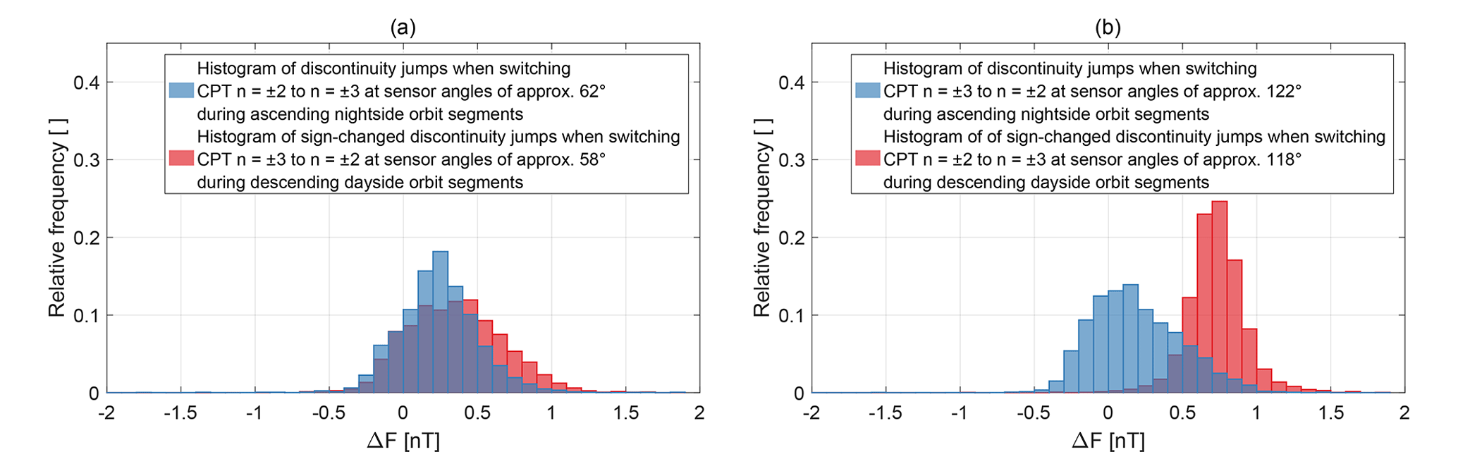
Figure 9 Histograms of the discontinuity jumps when switching the CPT resonance superpositions.

3.2.1 Discontinuity jumps when switching CPT resonance superpositions

Figure 9 shows the histograms for the discontinuity jumps for the entire available data set. The blue histogram in Fig. 9a describes the changes in the magnetic field strength read-out introduced by switching from the CPT resonance superposition $n=\pm \mathrm{2}$ to $n=\pm \mathrm{3}$ at sensor angles of approximately 62^∘ during nightside orbit segments. The blue histogram in Fig. 9b shows the discontinuity jumps when switching from the CPT resonance superposition $n=\pm \mathrm{3}$ to $n=\pm \mathrm{2}$ for nightside orbit segments which occur at sensor angles of approximately 122^∘. The red histogram in Fig. 9b describes the discontinuity jumps when switching from the CPT resonance superposition $n=\pm \mathrm{2}$ to $n=\pm \mathrm{3}$ at sensor angles of approximately 118^∘ during dayside orbit segments. The red histogram in Fig. 9a shows the discontinuity jumps when switching from the CPT resonance superposition $n=\pm \mathrm{3}$ to $n=\pm \mathrm{2}$ for dayside orbit segments which occur at sensor angles of approximately 58^∘. The sign of the values for the dayside orbit segments was changed to make them comparable to the nightside orbit segments for similar sensor angles. Ideally, each of the four medians should be zero. There is no significant difference between the medians of 0.34 and 0.23 nT when switching CPT resonance superpositions at approximately 58 and 62^∘, respectively. However, a significant difference exists when switching CPT resonance superpositions at approximately 118 and 122^∘ (0.72 and 0.15 nT, respectively).

3.2.2 Microwave oscillator detuning sensitivity of the magnetic field measurement

The sensitivity of the magnetic field measurement as a function of a microwave oscillator frequency detuning (from here on called detuning sensitivity) can be determined in orbit for measurements with the CPT resonance superposition $n=\pm \mathrm{2}$. As discussed in Sect. 2.1 every second is divided in three subsequent parts. During the second third of each second, the microwave oscillator frequency controller tracks the HFS ground state splitting. In the last third of each second, this controller is paused and the latest control value is adjusted by an offset in order to re-centre the microwave oscillator frequency with respect to the single CPT resonances $n=+\mathrm{2}$ and $n=-\mathrm{2}$. The CPT resonance n=0 and the CPT resonance superposition $n=\pm \mathrm{2}$ depend differently on the magnetic field strength in second order. The applied offset is half of this frequency difference and thus a function of the magnetic field strength. The control loop for the magnetic field measurement is active at all times, and read-outs can be derived during the microwave oscillator tracking and offset parts separately. In orbit the magnetic field strength changes with up to 40 nT s⁻¹, and therefore measurements done during the tracking part of each second have been interpolated to make them comparable with the offset part of each second. The impact on the magnetic field measurement as a function of the applied microwave controller offset can be used to calculate the detuning sensitivity.

Figure 10 Detuning sensitivity of the magnetic field measurement.

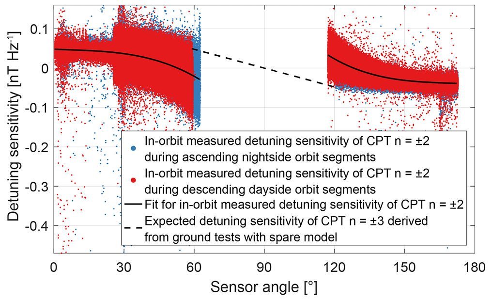
The blue and red dots in Fig. 10 show the calculated detuning sensitivity for in-orbit measurements with the CPT resonance superposition $n=\pm \mathrm{2}$. The detuning sensitivity depends on the sensor angle. Apart from data artefacts, the scatter of the measured detuning sensitivity is a function of the magnetic field strength. It is dominated by the division through the microwave oscillator controller offset and increases with decreasing magnetic field values and thus smaller offset values. This can be observed via the South Atlantic Anomaly, which keeps the noise level quite high towards lower sensor angles in the Southern Hemisphere during many orbits. It also explains the step-like drop of the noise at a sensor angle of 25^∘. The black solid lines are a fit of the in-orbit measurements whose shape was confirmed with the flight spare model on the ground.

For the measurements with the CPT resonance superposition $n=\pm \mathrm{3}$ the detuning sensitivity cannot be calculated from in-orbit data. The microwave oscillator controller cannot track the HFS ground state splitting, and the latest control value during measurements with the CPT resonance superposition $n=\pm \mathrm{2}$ is always adjusted by an offset as a function of the current magnetic field strength. The detuning sensitivity for measurements with the CPT resonance superposition $n=\pm \mathrm{3}$ shown in Fig. 10 was derived from measurements with the flight spare model.

The detuning sensitivity crosses zero at 53 and 127^∘ for measurements with the CPT resonance superposition $n=\pm \mathrm{2}$ and at 90^∘ for measurements with the CPT resonance superposition $n=\pm \mathrm{3}$. At these sensor angles the magnetic field measurement is not sensitive to the (offset) detuning of the microwave oscillator frequency with respect to the centre of the single CPT resonances $n=+\mathrm{2}$ and $n=-\mathrm{2}$ or $n=+\mathrm{3}$ and $n=-\mathrm{3}$.

Figure 11 Optical power during orbit segments.

Figure 12 Histograms of the optical power when switching the CPT resonance superpositions.

3.2.3 Optical power

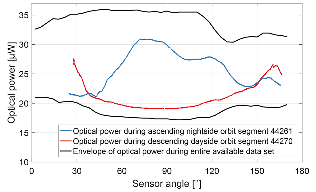
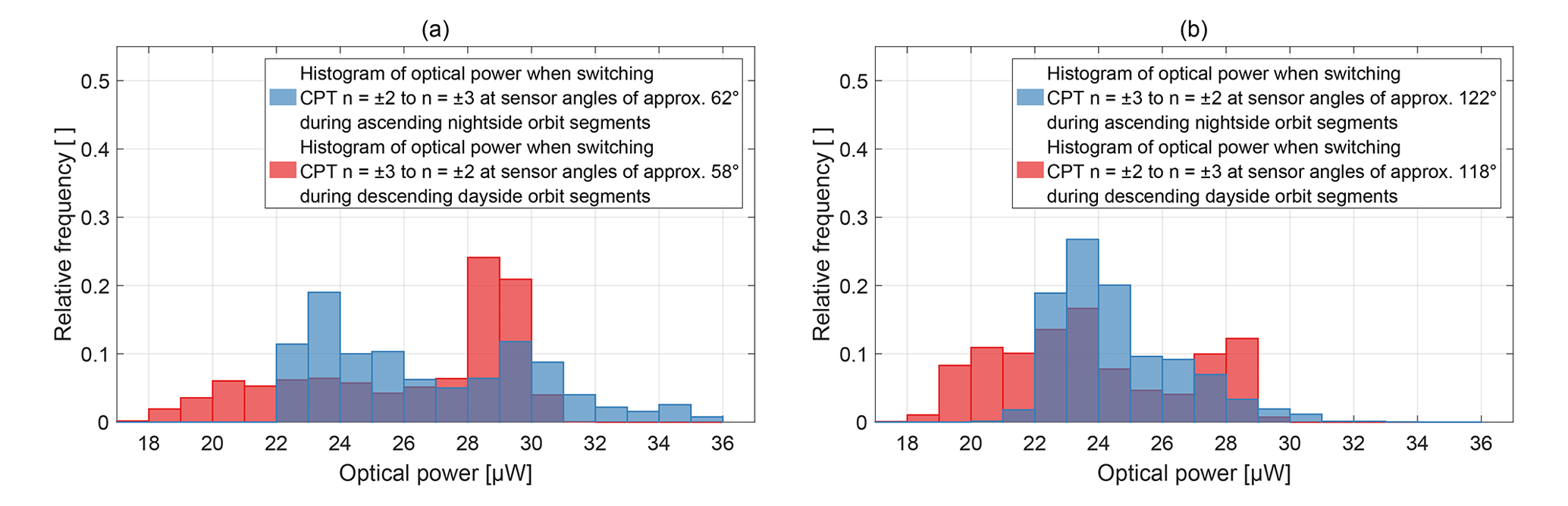
The black lines in Fig. 11 show the envelope of the optical power received at the photodiode for the entire available data set. It is proportional to the optical power in the sensor and varies between 17 and 36 µW due to the instrument design, as described in the Introduction. A major part of this variation occurs every orbit, which can be observed with the sample orbit segments 44261 and 44270. For completeness, Fig. 12 shows the histograms of the optical power when the CDSM switches between the resonance superpositions $n=\pm \mathrm{2}$ and $n=\pm \mathrm{3}$. As an example and similar to Fig. 9, the blue histogram in Fig. 12a describes the optical power when switching from the CPT resonance superposition $n=\pm \mathrm{2}$ to $n=\pm \mathrm{3}$ at sensor angles of approximately 62^∘ during nightside orbit segments.

Figure 13 Sensor temperature during orbit segments.

3.2.4 Sensor temperature

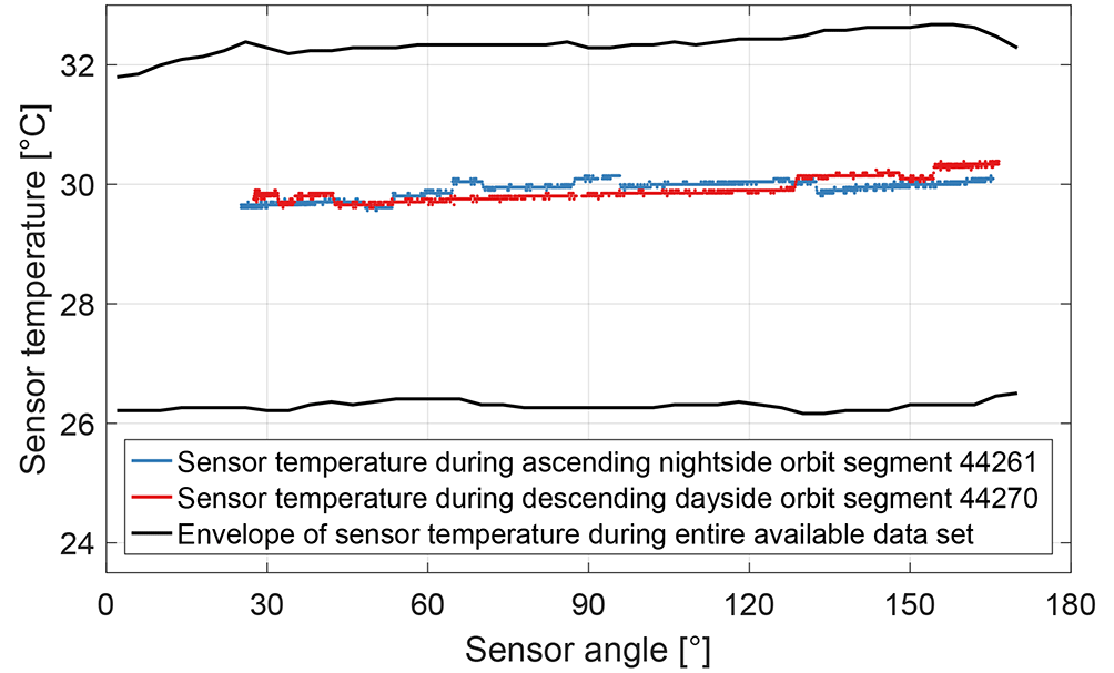
The black lines in Fig. 13 show the envelope of the sensor temperature for the entire available data set. The major part of the variation between 26.2 and 32.7 ^∘C is seasonal. The controller is not active and constant power heats the sensor unit. The same approach was used during the sensor heading characterization of the magnetic field measurement with the flight model on the ground (Pollinger et al., 2018) where the environmental temperature was settled within 0.1 ^∘C for each run. The in-orbit sensor temperature measurement experiences step-like interferences which can be observed with the sample orbit segments 44261 and 44270. These are likely caused by the unshielded twisted pair cable along the boom in combination with the high gain of the measurement circuit in order to minimize the current through the platinum resistance temperature detector close to the sensor cell. For further analysis the data were filtered.

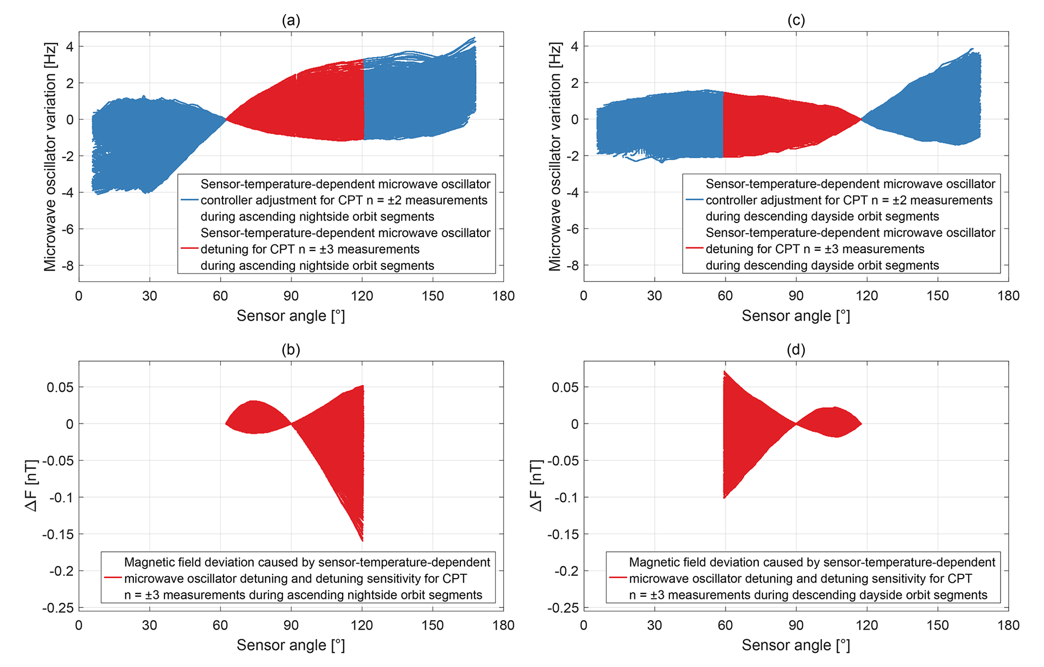
Figure 14 Sensor-temperature-dependent microwave oscillator variation and magnetic field deviation.

The HFS ground state splitting frequency depends on the sensor temperature with 13 Hz K⁻¹ (Pollinger et al., 2018). Figure 14a and c show the sensor-temperature-dependent variations of the microwave oscillator for the entire available data set. The variations are offset with respect to the reference points when switching from CPT resonance superposition $n=\pm \mathrm{2}$ to $n=\pm \mathrm{3}$, which occurs at the sensor angles of approximately 62 and 118^∘ for nightside and dayside orbit segments, respectively. For measurements with the CPT resonance superposition $n=\pm \mathrm{2}$ the microwave oscillator controller is active and can compensate for the sensor-temperature-dependent frequency changes in the HFS ground state splitting via the CPT resonance n=0. The adjustment values are shown as blue lines. For measurements with the CPT resonance superposition $n=\pm \mathrm{3}$ the microwave oscillator controller is paused and does not track the sensor-temperature-dependent frequency changes in the HFS ground state splitting. A temperature change leads to a detuning of the microwave oscillator frequency with respect to the centre of the single CPT resonances $n=+\mathrm{3}$ and $n=-\mathrm{3}$. This detuning is shown in Fig. 14a and c as red lines with a maximum detuning of 3.3 and −2.1 Hz for nightside and dayside orbit segments, respectively. In combination with the detuning sensitivity discussed in Fig. 10 the detuning can cause a deviation of the magnetic field measurement with the CPT resonance superposition $n=\pm \mathrm{3}$. The derived magnetic field deviation is shown in Fig. 14b and d with a maximum deviation of the magnetic field strength of −0.16 and −0.10 nT for nightside and dayside orbit segments, respectively. A sensor temperature change can contribute to the discontinuity jumps when switching from CPT resonance superposition $n=\pm \mathrm{3}$ to $n=\pm \mathrm{2}$ in Fig. 9 but cannot affect the discontinuity jumps when switching from CPT resonance superposition $n=\pm \mathrm{2}$ to $n=\pm \mathrm{3}$.

Figure 15 Reoccurring PCB temperature pattern during orbit segments.

3.2.5 PCB temperature and noise of the microwave oscillator control loop

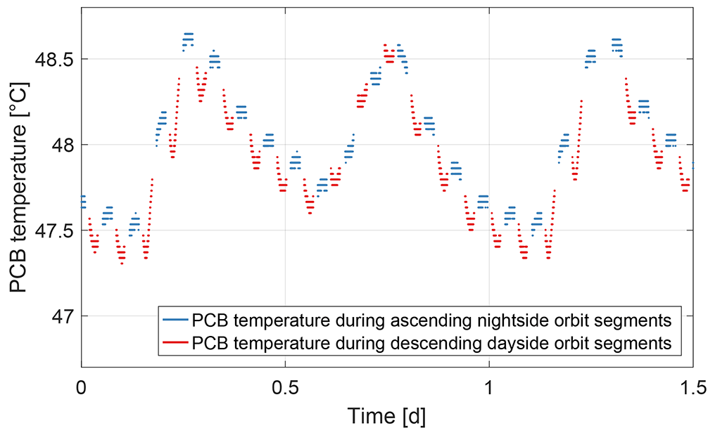
The temperature of the printed circuit board (PCB) is between 46.2 and 49.7 ^∘C for the entire available data set. It has a reoccurring pattern which is displayed for 1.5 d in Fig. 15. The maximum temperature change is 0.03 K min⁻¹, which occurs during specific dayside orbit segments.

The impact of the PCB temperature variations in space was investigated with the flight spare model on the ground. The microwave generator is realized by a phase-locked loop which consists of a voltage-controlled microwave oscillator and a fractional-N counter frequency divider (Pollinger et al., 2018). The time base for the microwave oscillator is an adjustable reference oscillator which is tuned via a voltage input by the actuating variable of the microwave oscillator controller. The reference oscillator is temperature-compensated and autonomously adjusts the output as a function of the environmental temperature in order to mitigate the temperature dependence of the oscillator.

Figure 16 Temperature dependence of the microwave oscillator output frequency.

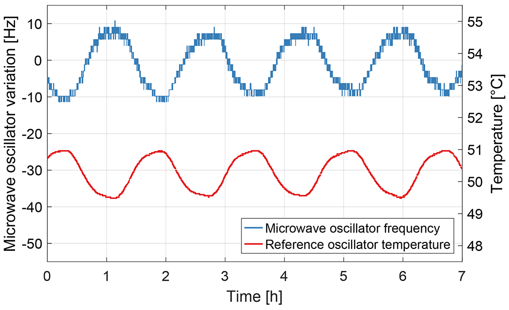
The temperature dependence of the reference oscillator was evaluated with the instrument box of the flight spare model located in the thermally controlled environment of a vacuum chamber. The output frequency was measured with a HP5335A counter and a SRS FS725 rubidium frequency standard. The instrument box and the counter were connected via an electrical vacuum feedthrough. The reference oscillator temperature was derived from the CDSM housekeeping data since the PCB temperature measurement is within 0.5 cm on the electronics board. The reoccurring pattern of the in-orbit PCB temperature cannot be reproduced exactly with the available test facilities. Figure 16 shows the frequency change for a temperature variation of 1.4 K within an orbit period of approximately 95 min and a maximum temperature change of 0.07 K min⁻¹. The reference oscillator frequency varies, which is equivalent to a change in the microwave oscillator frequency of −14.8 Hz K⁻¹.

The noise of the microwave oscillator control loop was evaluated with the instrument box of the flight spare model located in the thermally controlled environment of a vacuum chamber and the sensor unit positioned outside in a µ-metal shielding can. The instrument box and the sensor unit were connected via optical and electrical vacuum feedthroughs. The maximum duration of measurements with the CPT resonance superposition $n=\pm \mathrm{3}$ is 13 min during each orbit segment for the entire available data set. This is longer than each of the two measurement intervals with the CPT resonance superposition $n=\pm \mathrm{2}$ during each orbit segment for the entire available data set. The sensor temperature was controlled by the CDSM electronics, and the CDSM housekeeping read-out varied within 0.01 ^∘C for the evaluation period of 13 min. The PCB temperature was kept constant by the vacuum chamber, and the CDSM housekeeping read-out varied within 0.05 ^∘C for the evaluation period of 13 min. An artificial magnetic field was generated in the µ-metal shielding can with a Keithley 6221 current source and a coil. The generated magnetic field strength can be assumed to be sufficiently constant for this evaluation. The microwave oscillator controller tracked the CPT resonance n=0, and the actuating variable is a measure for the adjustment of the microwave oscillator output frequency. The standard deviation σ of the calculated microwave oscillator output frequency is 0.6 Hz for the evaluation period of 13 min.

Figure 17 PCB-temperature-dependent microwave oscillator variation and magnetic field deviation.

Figure 17a and c show PCB-temperature-dependent variations of the microwave oscillator for the entire available data set. The analysis for the adjustment and detuning values is identical to the sensor temperature. The variations are offset with respect to the reference points when switching from CPT resonance superposition $n=\pm \mathrm{2}$ to $n=\pm \mathrm{3}$. The adjustment for measurements with the CPT resonance superposition $n=\pm \mathrm{2}$ is shown as blue lines, while the detuning for measurements with the CPT resonance superposition $n=\pm \mathrm{3}$ is displayed as red lines. The derived magnetic field deviation for measurements with the CPT resonance superposition $n=\pm \mathrm{3}$ is shown in Fig. 17b and d. The maximum detuning of 1.0 and −2.1 Hz leads with the angular-dependent detuning sensitivity to a maximum deviation of the magnetic field values of −0.05 and −0.10 nT for nightside and dayside orbit segments, respectively. A PCB temperature change can contribute to the discontinuity jumps when switching from CPT resonance superposition $n=\pm \mathrm{3}$ to $n=\pm \mathrm{2}$ in Fig. 9 but cannot affect the discontinuity jumps when switching from CPT resonance superposition $n=\pm \mathrm{2}$ to $n=\pm \mathrm{3}$.

Figure 18 Angular-dependent microwave oscillator adjustment during ground tests.

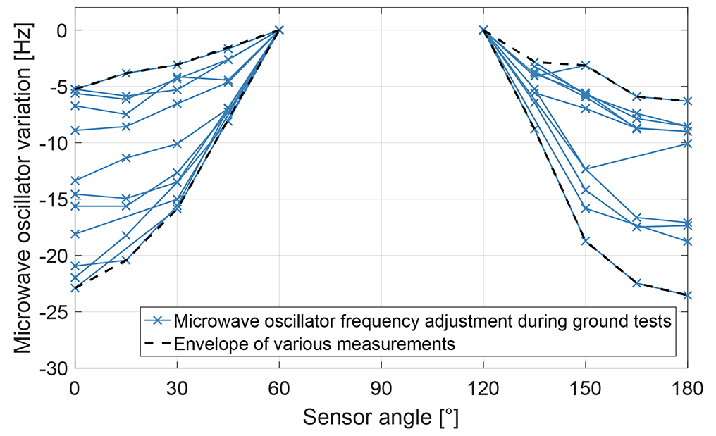
3.2.6 Angular-dependent microwave oscillator adjustment during ground tests

An angular-dependent adjustment of the microwave oscillator frequency could be observed for measurements with the CPT resonance superposition $n=\pm \mathrm{2}$. The data in Fig. 18 were derived during the sensor heading characterization of the magnetic field measurement with the flight model on the ground. The blue lines show individual measurements at the Conrad Observatory (COBS) of the Zentralanstalt für Meteorologie und Geodynamik in Lower Austria and in the coil systems of the Technical University Braunschweig (TU-BS) in Germany as well as the Fragment Mountain Weak Magnetic Laboratory of the National Institute of Metrology (NIM) in China (see Fig. 4b). The microwave oscillator variations are referenced to the sensor angles of 60 and 120^∘ in order to make them comparable. The black dashed lines show the envelope of these measurements. The microwave oscillator adjustment varies between −5 and −24 Hz. The sensor and PCB temperatures were settled within 0.1 ^∘C for each run, which would lead to an adjustment of the microwave oscillator frequency of only 0.7 and 1.5 Hz, respectively. The magnetic field strength was artificially controlled for the measurements at TU-BS and NIM. A magnetic field variation of 20 nT at an Earth field of 48 550 nT would lead to an adjustment of the microwave oscillator frequency of just 0.06 Hz during the COBS measurements. Thus, the reason for the angular-dependent behaviour cannot be explained so far.

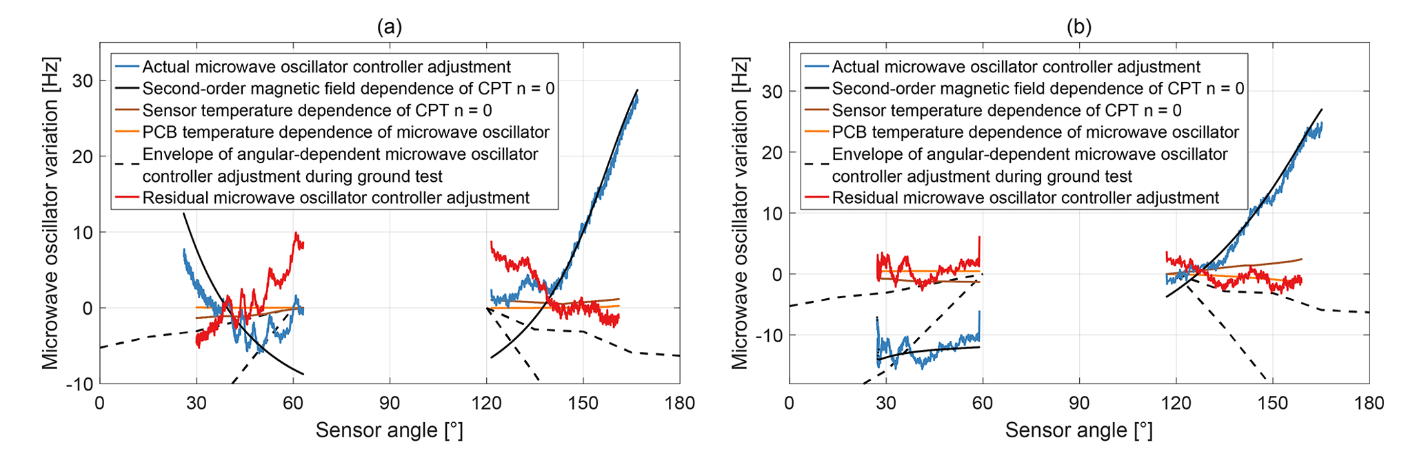
Figure 19 Microwave oscillator variation during measurements with the CPT resonance superposition $n=\pm \mathrm{2}$ for individual orbit segments.

3.2.7 Unknown residual microwave oscillator adjustment and derived uncertainty of magnetic field measurement

Figure 19 shows two examples of microwave oscillator variations during measurements with the CPT resonance superposition $n=\pm \mathrm{2}$ in orbit. The blue curves display the actual microwave oscillator controller adjustment required to track the CPT resonance n=0 with the microwave oscillator frequency. The re-centring as described in Sect. 2.1 is not displayed for simplicity. The output frequency is offset to the last microwave oscillator controller value before it was paused when switching from CPT resonance superposition $n=\pm \mathrm{2}$ to $n=\pm \mathrm{3}$. For the ascending nightside orbit segment 44261 in Fig. 19a and the descending dayside orbit segment 44270 in Fig. 19b this occurred at 62 and 118^∘, respectively. The brown and orange lines are the calculated microwave oscillator adjustments needed to compensate for the sensor and PCB temperature changes with respect to the reference point when switching from CPT resonance superposition $n=\pm \mathrm{2}$ to $n=\pm \mathrm{3}$. The black solid lines are the expected frequency change in the CPT resonance n=0 as a function of the magnetic field strength in second order. Their vertical offset was obtained by nonlinear least-squares fitting to the actual microwave oscillator controller adjustment for each individual orbit segment. The envelope of the angular-dependent microwave oscillator adjustment discovered during ground tests is shown as black dashed lines. The influences of the magnetic field strength in second order, the sensor temperature and the PCB temperature are understood and can be subtracted from the actual microwave oscillator controller adjustment. The residuals between the actual and understood microwave oscillator adjustments are plotted as red lines in Fig. 19 and show the same sensor angular-dependent trend as the ground measurements in Fig. 18.

Figure 20 Residual microwave oscillator adjustment for measurements with the CPT resonance superposition $n=\pm \mathrm{2}$.

The residual microwave oscillator controller adjustments vary with each orbit segment. Figure 20 shows the residuals for the entire available data set. The maximum residual microwave oscillator adjustment is 17.3 Hz and occurs during nightside orbit segments.

Figure 21 Derived uncertainty of magnetic field measurement as a function of the sensor angle.

For measurements with the CPT resonance superposition $n=\pm \mathrm{2}$ it can be assumed that the controller adjusts the microwave oscillator frequency correctly to the CPT resonance n=0 with the limit of the control loop noise discussed above. Since the cause of the residual microwave oscillator adjustment in Fig. 20 is unknown, it cannot be assumed that the offset-adjusted light field matches the centre of the single CPT resonances $n=+\mathrm{2}$ and $n=-$2 for measurements with the CPT resonance superposition $n=\pm \mathrm{2}$. A theoretical magnetic field deviation associated with the residual microwave oscillator adjustment can be calculated via the detuning sensitivity for measurements with the CPT resonance superposition $n=\pm \mathrm{2}$ in Fig. 10. This deviation is shown as blue and red dots in Fig. 21. Taking the maximum residual microwave oscillator adjustment and the detuning sensitivity for measurements with the CPT resonance superposition $n=\pm \mathrm{2}$, one can derive an uncertainty for the magnetic field measurements with the CPT resonance superposition $n=\pm \mathrm{2}$ for the available 9387 orbit segments. In Fig. 21 this uncertainty is visualized with solid black lines and grey areas below for sensor angles between approximately 6 and 62^∘ as well as 118 and 169^∘. The maximum derived uncertainty for measurements with the CPT resonance superposition $n=\pm \mathrm{2}$ is ±0.8 nT.

As mentioned above, for the measurements with the CPT resonance superposition $n=\pm \mathrm{3}$ the microwave oscillator control loop is paused when switching from CPT resonance superposition $n=\pm \mathrm{2}$ to $n=\pm \mathrm{3}$, and the last control value is offset as a function of the current magnetic field strength. The influence of the sensor and PCB temperature changes during measurements with the CPT resonance superposition $n=\pm \mathrm{3}$ could be mitigated with correction curves. Temperature-dependent correction terms could be additionally applied to the last control value in order to compensate for a change in the HFS ground state splitting or a temperature drift of the microwave oscillator frequency. This is implemented in the flight model but would require a regular update of certain parameters, which is not applicable for this mission. The uncertainties of the magnetic field measurement caused by sensor and PCB temperature changes without correction terms are shown in Fig. 21 as brown and orange areas, respectively. The uncertainties were defined as the absolute maximum deviations in Fig. 14b and d as well as Fig. 17b and d as a function of the sensor angle.

With the observed residual microwave oscillator adjustment during measurements with the CPT resonance superposition $n=\pm \mathrm{2}$ it can be assumed that similar additional adjustments would be required to re-centre the light field with respect to the single CPT resonances $n=+\mathrm{3}$ and $n=-\mathrm{3}$ during measurements with the CPT resonance superposition $n=\pm \mathrm{3}$. Taking the maximum residual microwave oscillator adjustment during measurements with the CPT resonance superposition $n=\pm \mathrm{2}$ and the expected detuning sensitivity for measurements with the CPT resonance superposition $n=\pm \mathrm{3}$ one can calculate a theoretical uncertainty associated with the expected microwave oscillator detuning during measurements with the CPT resonance superposition $n=\pm \mathrm{3}$. In Fig. 21 this uncertainty is visualized as grey areas for sensor angles between approximately 58 and 122^∘ .

The sum of the sensor-temperature-dependent uncertainty, the PCB-temperature-dependent uncertainty and the uncertainty derived from the expected microwave oscillator detuning during measurements with the CPT resonance superposition $n=\pm \mathrm{3}$ can be interpreted as the uncertainty of the magnetic field measurement with the CPT resonance superposition $n=\pm \mathrm{3}$. The derived uncertainty does not exceed ±1.1 nT and is displayed in Fig. 21 with black dashed lines. The derived uncertainty of the magnetic field measurement as a function of geomagnetic coordinates is shown in Fig. 22.

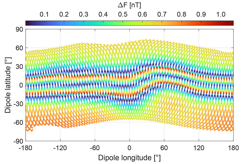
Figure 22 Derived uncertainty of the magnetic field measurement as a function of geomagnetic coordinates.

With the results of Fig. 21 one can calculate the sum of the derived uncertainties for the magnetic field measurement with the CPT resonance superpositions $n=\pm \mathrm{2}$ and $n=\pm \mathrm{3}$ for sensor angles when the CPT resonance superpositions $n=\pm \mathrm{2}$ and $n=\pm \mathrm{3}$ are switched (see Sect. 3.2.1). The combined uncertainties for the magnetic field measurement are approximately ±1.4, ±1.4, ±1.5 and ±1.4 nT at the sensor angles of approximately 58, 62, 118 and 122^∘, respectively; 99.3 %, 99.3 %, 99.5 % and 99.8 % of the corresponding discontinuity jumps are within the combined derived uncertainties for the magnetic field measurement with the CPT resonance superpositions $n=\pm \mathrm{2}$ and $n=\pm \mathrm{3}$.

4 Conclusions

The China Seismo-Electromagnetic Satellite (CSES) mission provides the first demonstration of the Coupled Dark State Magnetometer (CDSM) measurement principle in space. The CDSM is operational and all available housekeeping data have been nominal throughout the elapsed mission time.

Data correction processes were established in order to improve the accuracy of the CDSM data. This includes the extraction of valid 1 Hz data, the application of the sensor heading characteristic, the handling of discontinuities, which occur when switching between the coherent population trapping (CPT) resonance superpositions, and the removal of fluxgate and satellite interferences. The sum of all corrections applied to the CDSM L1 data is between −2.4 and 3.6 nT.

The CDSM measurements were compared to the Absolute Scalar Magnetometer (ASM) measurements aboard the Swarm satellite Bravo via the CHAOS-6 Earth field model between 15 and 30 November 2018. In this period the ascending nodes of the Swarm satellite Bravo were between 02:38 and 01:19 and 48–42 min after the ascending nodes of CSES at 02:00. The local time ranges overlapped. For nightside orbit segments the mean values of both instrument deviations compared to the CHAOS-6 model were $\stackrel{\mathrm{‾}}{\mathrm{\Delta }F}=\mathrm{1.5}$ nT for CDSM and $\stackrel{\mathrm{‾}}{\mathrm{\Delta }F}=\mathrm{0.9}$ nT for ASM in the magnetic dipole latitude range of −40 to −30^∘ (southern evaluation interval). For the dipole latitude range of 30 to 40^∘ (northern evaluation interval) the mean values of both instruments differed by 1.9 nT ($\stackrel{\mathrm{‾}}{\mathrm{\Delta }F}=\mathrm{2.7}$ nT for CDSM and $\stackrel{\mathrm{‾}}{\mathrm{\Delta }F}=\mathrm{0.8}$ nT for ASM). Similar differences between the CDSM and the ASM mean values were also observed for dayside orbit segments.

For the available data set of 9387 orbit segments, discontinuity jumps with a median up to 0.72 nT were observed in the magnetic field strength read-out when the CDSM switched between the CPT resonance superpositions $n=\pm \mathrm{2}$ and $n=\pm \mathrm{3}$. All available instrument parameters, especially the microwave oscillator frequency controller adjustment, were investigated in detail. The frequency of the microwave oscillator is used to track the hyperfine structure (HFS) ground state splitting via the CPT resonance n=0 and is part of the light field to track the CPT resonance superposition $n=\pm \mathrm{2}$ or $n=\pm \mathrm{3}$ for the magnetic field measurement. The sensitivity of the magnetic field measurement on a microwave oscillator frequency detuning was calculated from in-orbit measurements with the CPT resonance superposition $n=\pm \mathrm{2}$. For measurements with the CPT resonance superposition $n=\pm \mathrm{3}$ this detuning sensitivity was determined with the flight spare model on the ground.

During measurements with the CPT resonance superposition $n=\pm \mathrm{3}$, the microwave oscillator control loop is paused and cannot track changes in the sensor and PCB temperatures. The maximum deviations of the magnetic field measurement caused by sensor and PCB temperature changes during measurements with the CPT resonance superposition $n=\pm \mathrm{3}$ were absolute 0.16 and 0.10 nT, respectively, for the available data set in orbit.

During measurements with the CPT resonance superposition $n=\pm \mathrm{2}$, the microwave oscillator control loop tracks changes in the HFS ground state splitting caused by variations of the magnetic field strength in second order or the sensor temperature, and it compensates for a possible temperature-dependent drift of the electronics. These influences are understood and can be subtracted from the actual microwave oscillator controller adjustment. A residual microwave controller adjustment up to 17.3 Hz could be observed for the available data set of 9387 orbit segments. With the maximum of this residual microwave oscillator adjustment and the calculated detuning sensitivity one can derive an uncertainty of the magnetic field measurement, which depends on the sensor angle between the light propagation direction through the sensor and the magnetic field vector. This derived uncertainty does not exceed ±0.8 nT for measurements with the CPT resonance superposition $n=\pm \mathrm{2}$ and ±1.1 nT for measurements with the CPT resonance superposition $n=\pm \mathrm{3}$. It is zero at sensor angles of 53, 90 and 127^∘. At these angles the magnetic field measurement is not sensitive to a moderate detuning of the microwave oscillator frequency with respect to the centre of the single CPT resonances $n=+\mathrm{2}$ and $n=-\mathrm{2}$ or $n=+\mathrm{3}$ and $n=-\mathrm{3}$.

For future missions a new sensor design is under development with which the light field passes the Rb-filled glass cell twice but with opposite helicities of the circular polarization state (Ellmeier, 2019). This reduces the sensitivity of the magnetic field measurement to the microwave oscillator frequency detuning.