the Creative Commons Attribution 4.0 License.
the Creative Commons Attribution 4.0 License.
 | 28 Jun 2021
A comparison of gap-filling algorithms for eddy covariance fluxes and their drivers
Jason Beringer
Matthias Leopold
Ian McHugh
James Cleverly
Peter Isaac
Azizallah Izady
The errors and uncertainties associated with gap-filling algorithms of water, carbon, and energy fluxes data have always been one of the main challenges of the global network of microclimatological tower sites that use the eddy covariance (EC) technique. To address these concerns and find more efficient gap-filling algorithms, we reviewed eight algorithms to estimate missing values of environmental drivers and nine algorithms for the three major fluxes typically found in EC time series. We then examined the algorithms' performance for different gap-filling scenarios utilising the data from five EC towers during 2013. This research's objectives were (a) to evaluate the impact of the gap lengths on the performance of each algorithm and (b) to compare the performance of traditional and new gap-filling techniques for the EC data, for fluxes, and separately for their corresponding meteorological drivers. The algorithms' performance was evaluated by generating nine gap windows with different lengths, ranging from a day to 365 d. In each scenario, a gap period was chosen randomly, and the data were removed from the dataset accordingly. After running each scenario, a variety of statistical metrics were used to evaluate the algorithms' performance. The algorithms showed different levels of sensitivity to the gap lengths; the Prophet Forecast Model (FBP) revealed the most sensitivity, whilst the performance of artificial neural networks (ANNs), for instance, did not vary as much by changing the gap length. The algorithms' performance generally decreased with increasing the gap length, yet the differences were not significant for windows smaller than 30 d. No significant differences between the algorithms were recognised for the meteorological and environmental drivers. However, the linear algorithms showed slight superiority over those of machine learning (ML), except the random forest (RF) algorithm estimating the ground heat flux (root mean square errors – RMSEs – of 28.91 and 33.92 for RF and classic linear regression – CLR, respectively). However, for the major fluxes, ML algorithms and the MDS showed superiority over the other algorithms. Even though ANNs, random forest (RF), and eXtreme Gradient Boost (XGB) showed comparable performance in gap-filling of the major fluxes, RF provided more consistent results with slightly less bias against the other ML algorithms. The results indicated no single algorithm that outperforms in all situations, but the RF is a potential alternative for the MDS and ANNs as regards flux gap-filling.
- Article
(1885 KB) - Full-text XML
-
Supplement
(423 KB) - BibTeX
- EndNote


To address the global challenges of climatological and ecological changes, environmental scientists and policy makers are demanding data that are continuous in time and space. In addition, there is a need to quantify and reduce uncertainties in such data, including observations of carbon, water, and energy exchanges that are crucial components in national and international flux networks as well as global Earth-observing systems. Satellites partially fill this gap as they provide excellent spatial coverage but have limited temporal resolution and do not measure at a point scale. As such, high-quality long-term site observations of ecosystem processes and fluxes are needed that are continuous in time and space. The global eddy covariance (EC) flux tower network (FLUXNET) consists of its regional counterparts (i.e. AmeriFlux, EUROFLUX, OzFlux) and was established in the late 1990s to address the global demand for such information (Aubinet et al., 1999; Baldocchi et al., 2001; Beringer et al., 2016; Hollinger et al., 1999; Menzer et al., 2013; Tenhunen et al., 1998). Despite EC data being frequently used to validate process modelling analyses, field surveys, and remote sensing assessments (Hagen et al., 2006), there are some serious concerns regarding the technique's challenges, e.g. data gaps and uncertainties. Hence, filling data gaps and reducing uncertainties through better gap-filling techniques are highly needed.
Even though the EC is a common technique to measure fluxes of carbon, water, and energy, there are some challenges in providing robust, high-quality, continuous observations. One of the challenges regarding the technique and therefore the flux networks is addressing data gaps and the uncertainties associated with the gap-filling process, mainly when the gap windows are long (longer than 12 consecutive days, as described by Moffat et al., 2007). These gaps happen quite often for a variety of reasons, such as values out of range, spike detection or manual exclusion of date and time ranges, instrument or power failure, herbivores, fire, eagles' nests, lightning, and/or researchers on leave (Beringer et al., 2017). Since EC flux towers are often located in harsh climates, their data are more susceptible to adverse weather (i.e. rain conditions), and they sometimes prevent quick access to sites for repair and maintenance. As a result, this issue can, in turn, produce gaps which might be relatively long (Isaac et al., 2017) and thus problematic, as explained in the following. Firstly, loss of data is considered a threat to scientific studies depending on the missing data quantity, pattern, mechanism, and nature (Altman and Bland, 2007; Molenberghs et al., 2014; Tannenbaum, 2010). That is because using an incomplete dataset might lead to biased, invalid, and unreliable results (Allison, 2000; Kang, 2013; Little, 2002). Second, continuous gap-filled data are required to calculate the annual or monthly budgets of carbon and water balance components (Hutley et al., 2005).
Other than the challenges caused by missing data, there are several sources of errors and uncertainties in the EC technique. Firstly, random error is associated with the stochastic nature of turbulence, associated sampling errors (incomplete sampling of large eddies, uncertainty in the calculated covariance between the vertical wind velocity and the scalar of interest), instrument errors, and footprint variability (Aubinet et al., 2012). For instance, Dragoni et al. (2007) analysed EC-based data from the Morgan–Monroe State Forest for 8 years (1999–2006) and assessed instrument uncertainty as equal to 3 % of the total annual net ecosystem exchange (NEE). Another primary source of uncertainty in EC measurements is systematic errors caused by methodological challenges and instrument calibration problems (e.g. sonic anemometer errors, spikes, gas analyser errors). Finally, one of the sources of uncertainties is data processing, especially data gap-filling (Isaac et al., 2017; Moffat et al., 2007; Richardson et al., 2012; Richardson and Hollinger, 2007).
There are several uncertainties pertaining to gap-filling of missing values, including measurement uncertainty (Richardson and Hollinger, 2007), lengths and timing of the gaps (Falge et al., 2001; Richardson and Hollinger, 2007), and the particular gap-filling algorithm that is used (Falge et al., 2001; Moffat et al., 2007). However, there are two dominant issues with long data gaps and the choice of a particular gap-filling algorithm (Aubinet et al., 2012). Firstly, long gaps can significantly increase the total amount of uncertainty as the ecosystem behaviour might change because of different agricultural periods or phenological phases (e.g. growing season, harvest period, bushfire) and thereby show different responses under similar meteorological conditions (Aubinet et al., 2012; Isaac et al., 2017; Richardson and Hollinger, 2007). Consequently, the period in which a long gap happens is important. For example, research undertaken by Richardson and Hollinger (2007) on data from a range of FLUXNET sites revealed that a week data gap during spring green-up in a forest led to a higher uncertainty over a 3-week gap period during winter. Second, each gap-filling algorithm has its strengths and weaknesses; for instance, Moffat et al. (2007) compared 15 different commonly used gap-filling algorithms. They found no significant difference between the performance of the algorithms with “good” reliability based on analysis of variance of the root mean square error (RMSE). The overall gap-filling uncertainty was within ±25 g C m−2 yr−1 for most of the proper algorithms, whereas the other algorithms generated higher uncertainties of up to ±75 g C m−2 yr−1, showing that the uncertainty provided by reliable methods can be considerably smaller. This result is similar to the findings of Richardson and Hollinger (2007), who found that for the datasets used in their study that uncertainties of up to ±30 g C m−2 yr−1 were from long gaps by appropriate algorithms. Considering that the data provided by EC tower networks are of use for research, government, and policy makers, robust gap-filling is a need to quantify and reduce uncertainties in flux estimations.
Several methods have typically been used to fill data gaps in both fluxes and their meteorological drivers to manage the missing data problem. Due to computational constraints of complex algorithms, early works to impute EC data gaps used interpolation methods based mostly on linear regression or temporal autocorrelation (Falge et al., 2001; Lee et al., 1999). These approaches were quickly replaced by more sophisticated methods such as non-linear regressions (Barr et al., 2004; Falge et al., 2001; Moffat et al., 2007; Richardson et al., 2006), look-up tables (Falge et al., 2001; Law et al., 2002; Zhao and Huang, 2015), artificial neural networks (ANNs) (Aubinet et al., 1999; Beringer et al., 2016; Cleverly et al., 2013; Hagen et al., 2006; Isaac et al., 2017; Kunwor et al., 2017; Moffat et al., 2007; Papale and Valentini, 2003; Pilegaard et al., 2001; Staebler, 1999), mean diurnal variation (Falge et al., 2001; Moffat et al., 2007; Zhao and Huang, 2015), and multiple imputations (Hui et al., 2004; Moffat et al., 2007). Each of these methods has its pros and cons as follows: (a) interpolation methods such as the mean diurnal variation (MDV) do not need any drivers, yet their accuracy is lower than other approaches (Aubinet et al., 2012). Moreover, this method may provide biased results on extremely clear or cloudy days (Falge et al., 2001). MDV is not recommended when a gap is longer than 2 weeks because it cannot consider the non-linear relations between the drivers and the flux, leading to a high level of uncertainty (Falge et al., 2001). (b) The look-up table, especially its modified version – marginal distribution sampling (MDS) – has provided performance close to ANNs and is more reliable and consistent than the other algorithms so far. Hence, MDS was chosen as one of the standard gap-filling methods in EUROFLUX (Aubinet et al., 2012). Nevertheless, the performance of MDS in gap-filling of extra long gaps is not well known (Kim et al., 2020). (c) ANNs have commonly been used to gap-fill EC fluxes since 2000, and because of their robust and consistent results they are considered a standard gap-filling algorithm in several networks, e.g. ICOS, FLUXNET, and OzFlux (Aubinet et al., 2012; Beringer et al., 2017; Isaac et al., 2017). Despite their reliable performance, ANNs – and generally all other ML algorithms – face some challenges. Over-fitting, for instance, is a big concern and can happen when the number of degrees of freedom is high, while the training window is not long enough or the quality of the training dataset is low. This challenge becomes acute when the gaps happen while the ecosystem behaviour is changing and shows different responses under similar meteorological conditions. Furthermore, there is a desire to have the training windows short so that the algorithm can track the ecosystem behaviour shift. Yet, this increases the risk of over-fitting depending on the algorithm. In other words, the training window length should be neither so short that it causes over-fitting nor so long that it leads to algorithms ignoring ecological condition changes. Long gaps are considered one of the primary uncertainty sources of CO2 flux in FLUXNET (Aubinet et al., 2012). As a result, studying the effects of the gap lengths and studying the window length whereby an algorithm is trained are both critical challenges associated with environmental data gap-filling.
Apart from the limitations and disadvantages of the mentioned algorithms, gap-filling of fluxes (e.g. NEE) experiences some other challenges that make it necessary to find or develop new gap-filling algorithms. That is because the current methods are not flexible enough to perform well on special occasions or with extreme values (Kunwor et al., 2017), and there is almost no room to optimise them to improve their outcome (Moffat et al., 2007). Moreover, even using the best available algorithm, such as ANNs, the model (gap-filling) uncertainty still accounts for a sizable proportion of the total uncertainties, especially when the gaps are relatively long. Since the 2000s when MDS and ANNs were chosen as the most reliable gap-filling methods for EC flux observations, many new ML and optimisation algorithms have been developed and used in various scientific fields. Some have shown superiority over ANNs, either individually or as a part of a hybrid or ensemble model (e.g. Gani et al., 2016). As a result, comparing the cutting-edge algorithms with the current standard ones can show whether there is any room to improve the gap-filling process within the field. According to the concerns mentioned above, this paper has two objectives: (a) to find out the impact of different gap lengths on the performance of each algorithm and (b) to compare the performance of traditional with new gap-filling techniques separately for fluxes and their meteorological drivers, particularly soil moisture, because this has always been a challenging variable to gap-fill due to the biology and heterogeneity of soil parameters. To address these objectives, we utilised nine different algorithms – eXtreme Gradient Boost (XGB), random forest (RF) algorithm, artificial neural networks (ANNs), marginal distribution sampling (MDS), classic linear regression (CLR), support vector regression (SVR), elastic net regularisation (ELN), panel data (PD), and the Prophet Forecast Model (FBP) – to fill the gaps of the major fluxes and eight of them (excluding MDS) to fill the gaps of the environmental drivers. We then assessed their relative performance to evaluate potentially better ways to fill EC flux data. To test the approaches, we used five flux towers from the OzFlux network. To evaluate the performance of these algorithms, nine scenarios for gaps were planned – from a day to a whole year – and applied to the datasets, and different common performance metrics (e.g. RMSE, MBE) and visual graphs were used.
In order to address the first objective of this research, nine different gap lengths were superimposed to the datasets, i.e. 1, 5, 10, 20, 30, 60, 90, 180, and 365 d. To address the second objective, we chose nine different algorithms to fill the gaps, including a wide variety of different approaches, e.g. from a simple algorithm like CLR to the cutting-edge ML algorithms like XGB (MDS was not used to gap-fill the environmental drivers). The data used in this paper came from five EC towers of the OzFlux network, i.e. Alice Springs Mulga, Calperum, Gingin, Howard Springs, and Tumbarumba, from 2012 to 2013, with a time resolution of 30 min, except for Tumbarumba (60 min). Additionally, data coming from three additional sources outside the network were also used as ancillary data to help the algorithms fill environmental driver gaps.
2.1 Data
The data used for this research came from OzFlux, which is the regional Australian and New Zealand flux tower network that aims to provide a continental-scale national research facility to monitor and assess Australia's terrestrial biosphere and climate (Beringer et al., 2016). As described in Isaac et al. (2017), all OzFlux towers continuously measure and record meteorological and flux variables at resolutions up to 10 Hz and use a 30 min averaging period, with a few exceptions (data are available from http://data.ozflux.org.au/portal, last access: 16 July 2018). The network acquires additional data from the Australian Bureau of Meteorology (BoM), the European Centre for Medium-Range Weather Forecasts (ECMWF), and the Moderate Resolution Imaging Spectroradiometer (MODIS) on the TERRA and AQUA satellites for alternative data for gap-filling flux tower datasets (Isaac et al., 2017). As explained by Isaac et al. (2017), OzFlux uses the BoM automated weather station (AWS) datasets to gap-fill the meteorological data, the BoM weather forecasting model (ACCESS-R) for radiation and soil data from 2011 onward, and MODIS MOD13Q1 for the normalised difference vegetation index (NDVI) and enhanced vegetation index (EVI). Moreover, the data provided by BIOS2, a physically based model–data integration environment for tracking Australian carbon and water (Haverd et al., 2015), were also used as another ancillary source for varieties of environmental features. Current ACCESS-R and MODIS data are available from the BoM OPeNDAP (http://www.opendap.org/, last access: 21 April 2018) server and TERN–AusCover data (http://www.auscover.org.au/, last access: 23 April 2018), respectively.
The datasets used in this research came from five towers from the OzFlux network between 2012 and 2013, each representative of a different climate and land cover for Australian ecological conditions (Alice Springs Mulga: tropical and subtropical desert, Calperum: steppe, Gingin: Mediterranean, Howard Springs: tropical savanna, Tumbarumba: oceanic; Table 1 and Beringer et al., 2016). The datasets included 15 meteorological drivers and three major fluxes recorded (Table 2) based upon the EC technique at a 30 min temporal resolution, except for Tumbarumba, which was hourly. Additionally, relevant ancillary datasets for the mentioned towers were used to follow the OzFlux network gap-filling protocol (Table 3). Each dataset was quality checked at three levels based on the OzFlux network protocol described in Isaac et al. (2017) and applied using PyFluxPro version 0.9.2. To address the underestimation of canopy respiration by EC measurements at night, we used the change-point detection (CPD) method (Barr et al., 2013) to reject nightly records when the friction velocity fell below each site's threshold value. After dismissing the inappropriate measurements, overall coverage of 72 %–88 % and 21 %–48 % was achieved for diurnal and nocturnal records during 2013 (the year to which the artificial gaps were superimposed), respectively.
Table 1Information on the five towers from which data were used, including their name, location, dominant species, and climate.

Table 2List of variables and their units used in this research, including the three main fluxes and their environmental drivers.
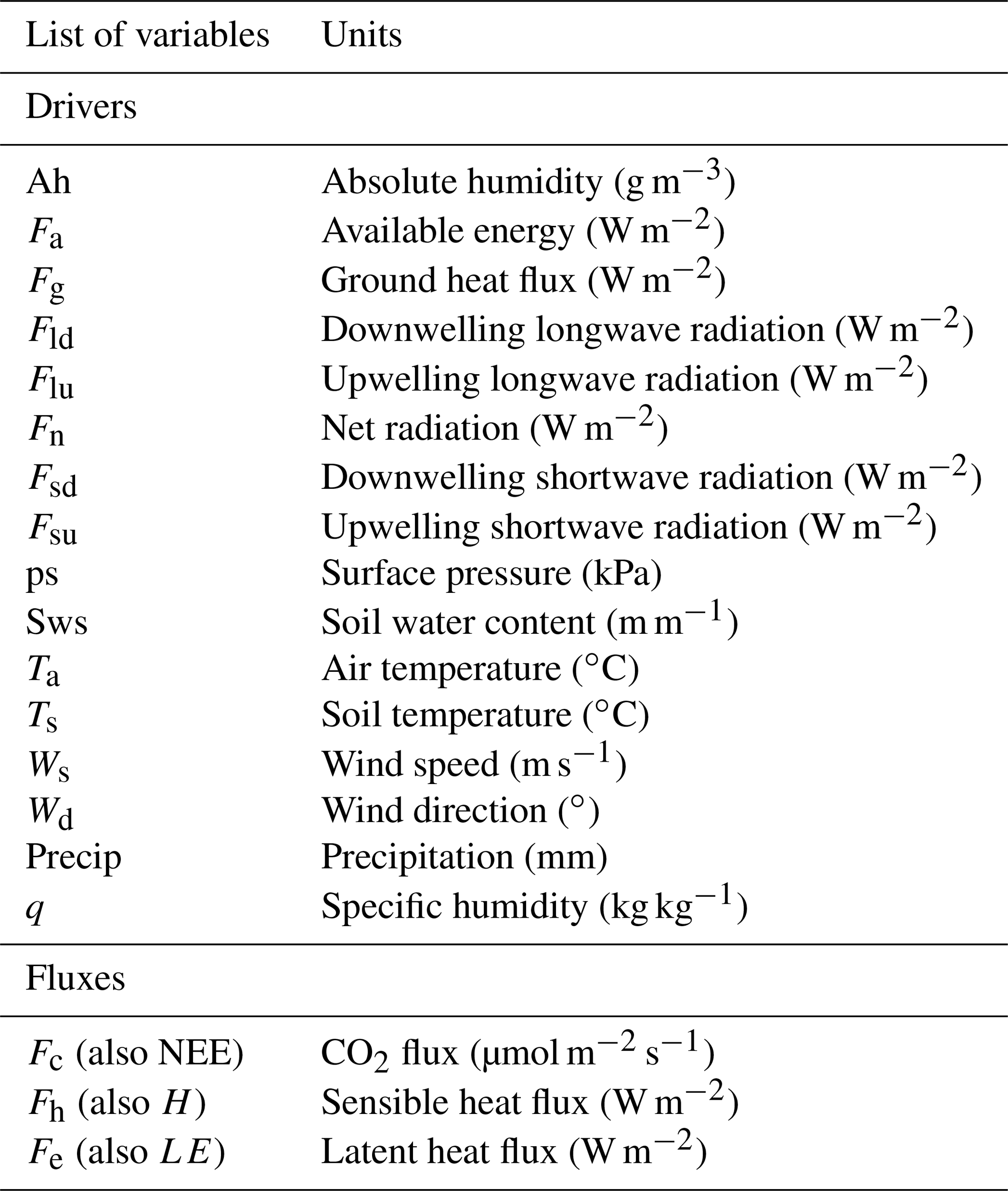
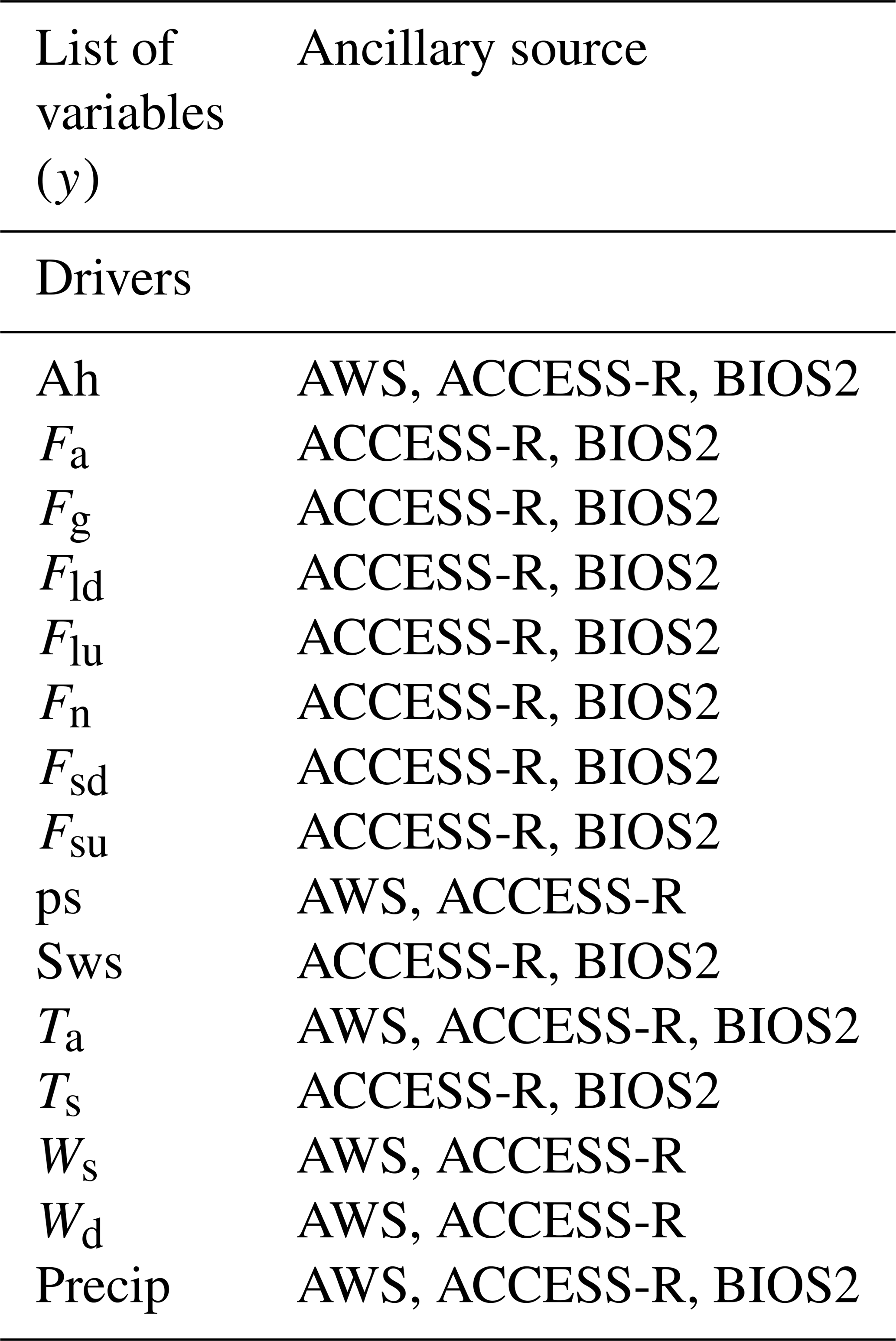
The datasets whereby each environmental variable was gap-filled are shown in Table 3. For each of these variables, the same variable of the ancillary source was used to fill the gaps. For instance, to gap-fill Ah, the Ah records of AWS, ACCESS-R, and BIOS2 were used. To gap-fill the missing values of fluxes, i.e. Fc (NEE), Fh (H), and Fe (LE), eight drivers were used as follows: Ta, Ws, Sws, Fg, vapour pressure deficit (VPD), Fn, q, and Ts based on a combination of random forest (RF) feature selection and testing out a series of feature combinations. Different Python programming language libraries (version 3.6.4) were utilised for training and testing the algorithms, i.e. XGBoost for XGB, fbprophet for FBP, statsmodels for PD, and sklearn for the rest of the algorithms. Each algorithm was tuned individually using a grid search, and the numbers of nodes, layers, and irritations were chosen accordingly.
Table 3The ancillary sources used to gap-fill each environmental driver.
2.2 Gap-filling algorithms
Eight imputation algorithms for estimating 15 environmental drivers and nine algorithms for the three major fluxes were chosen to make the comparison. These algorithms were selected in such a way that a variety of approaches were tested, from the standard methods like ANNs and MDS to the newer algorithms which have rarely or never been used in the field, such as eXtreme Gradient Boosting and panel data (Table 4).
Table 4The name and the abbreviation of the gap-filling algorithms.

2.2.1 Marginal distribution sampling (MDS)
Reichstein et al. (2005) introduced the MDS as an enhanced look-up table method, which considers both the covariation of fluxes with meteorological variables and the temporal autocorrelation of the fluxes (Aubinet et al., 2012). Alongside the ANNs, the MDS is considered one of the standard gap-filling methods for flux data amongst FLUXNET and is selected in this study to help the community have a clear idea of the performance of other algorithms. Unlike the other algorithms used in this research, we used Fsd, Ta, and VPD as the input features for the MDS to be consistent with standard application of the MDS; for using more than three or four drivers it is not generally recommended (Aubinet et al., 2012). The PyFluxPro version 0.9.2 was used to apply the algorithm (modified code used for gaps longer than 10 d).
2.2.2 Artificial neural networks (ANNs)
Rooted in the 1950s, artificial neural networks are ML methods inspired by biological neural networks and are classified as supervised learning methods (Dreyfus, 1990; Farley and Clark, 1954). ANNs work based on several connected units called nodes, which are used to mimic a neuron's functionality in an animal brain by sending and receiving signals to other nodes. The ANN technique used in this paper was the Multi-Layer Perceptron regressor, which optimises the squared loss using stochastic gradient descent. Sklearn.neural_network.MLPRegressor was used to apply this method in Python, and its hyperparameters were 800 and 500 for “hidden_layer_sizes” and “max_iter”, respectively, based on a grid search. ANNs are one of the current standard approaches for gap-filling in FLUXNET and in this research were picked out as a performance reference for other algorithms.
2.2.3 Classical linear regression (CLR)
A classical linear regression is an equation developed to estimate the value of the dependent variable (y) based on independent values (xi). In contrast, each xi has its specific coefficient and an overall intercept value. In this method, these coefficients are determined by minimising the squared residuals (errors) of estimated vs. observed values, called least squares. A CLR algorithm can be formulated as follows (Freedman, 2009):
where y is the dependent variable, α is the interception, Xi represent independent variables, βi is the coefficient of Xi, and ε is the error term. We chose this algorithm as a baseline to find out how much better more complicated algorithms can comparatively estimate dependent variables.
2.2.4 Random forests (RFs)
Random forest, a supervised ML algorithm used for both classification and regression, consists of multiple trees constructed systematically by pseudo-randomly selecting subsets of components of the feature vector: that is, trees constructed in randomly chosen subspaces (Ho, 1998). The RF algorithm has been developed to overcome the over-fitting problem, a commonplace limitation of its preceding decision-tree-based methods (Ho, 1995, 1998). Sklearn.ensemble.RandomForestRegressor was used to apply this method in Python, and the hyperparameters used were 5 and 1000 for “max_depth” and “n_estimators”, respectively, based on a grid search.
2.2.5 Support vector regression (SVR)
As a non-linear method, support vector regression was developed based on Vapnik's concept of support vector theory (Drucker et al., 1997). An SVR algorithm is trained by trying to solve the following problem:
where xi and yi are the training sample and target value in a row. The inner product plus intercept is the prediction for that sample, and ε is a free parameter that serves as a threshold. sklearn.svm.SVR was used to apply this method in Python, and the hyperparameters used were 1 and 0.001 for “C” and “γ”, respectively, based on a grid search.
2.2.6 Elastic net regularisation (ELN)
The elastic net is a linear regularised regression method that exerts small amounts of bias by adding two penalty components to the regressed line to decline the coefficients of independent variables. It thus provides better long-term predictions. Given that these two penalty components come from ridge regression and LASSO, the elastic net is considered a hybrid model consisting of ridge and LASSO regressions, thereby overcoming the limitations of both. The estimates from the ELN method can be formulated as below (Zou and Hastie, 2005):
where is the coefficient of each ELN independent variable, λ1 and λ2 are penalty coefficients of LASSO and ridge regression, respectively, is the coefficient of an independent variable calculated based on ordinary least squares, and “sgn” stands for the sign function:
The ELN regression is good at addressing situations when the training datasets have small samples or when there are correlations between parameters. sklearn.linear_model.ElasticNet was used to apply this method in Python, and the hyperparameters used were as follows: {“alpha”: 0.01, “fit_intercept”: True, “max_iter”: 5000, “normalize”: False} based on a grid search.
2.2.7 Panel data (PD)
The panel data method is a multidimensional statistical method mainly used in econometrics to analyse datasets which involve time series of observations amongst individual cross sections (Baltagi, 1995), usually based on ordinary least squares (OLS) or generalised least squares (GLS). A two-way panel data model consists of two extra components beyond a CLR as follows (Baltagi, 1995; Hsiao et al., 2002; Wooldridge, 2002):
where i and t denote the cross section and time series dimension in a row, y is a dependent-variable vector, X is an independent-variable matrix, α is a scalar, β is the coefficient of the independent-variable matrix, μi is the unobservable individual-specific effect, and λt is the unobservable time-specific effect. The panel data method has the ability to provide a holistic analysis of different individuals and determine the specific impact of every single time, which caused its superiority over CLR. Since PD requires cross sections to be applied, we used a cross section tower for each of the five main towers as follows: Ti Tree East for Alice Springs Mulga, Whroo for Calperum, Great Western Woodlands for Gingin, Daly River for Howard Springs, and Cumberland Plain for Tumbarumba. The cross section towers were chosen based on their distances (the closest ones with common years of data).
2.2.8 eXtreme Gradient Boost (XGB)
The eXtreme Gradient Boost algorithm is a reinforced method of gradient boost introduced in 1999 that works based on parallel boosted decision trees. Similar to RF, it can be used for a variety of data processing purposes including classification and regression (Friedman, 2001, 2002; Ye et al., 2009). The XGB method is resistant to over-fitting and provides a robust, portable, and scalable algorithm for large-scale boosting decision-tree-based techniques. sklearn.ensemble.GradientBoostingRegressor was used to apply this method in Python, and its hyperparameters were chosen based on a grid search as follows: {“learning_rate”: 0.001, “max_depth”: 8, “reg_alpha”: 0.1, “subsample”: 0.5}.
2.2.9 The Prophet Forecasting Model (FBP)
The Prophet Forecasting Model, also known as “Prophet”, is a time series forecasting model developed by Facebook to manage the common features of business time series. It is designed to have intuitive parameters that can be adjusted without knowing the details of the underlying model (Taylor and Letham, 2018). A decomposable time series model was used (Harvey and Peters, 1990) to develop this model, with three main components: trend, seasonality, and holidays (Taylor and Letham, 2018):
where g(t) is the trend function, which models non-periodic changes, s(t) is a function to represent periodic changes, e.g. seasonality, and h(t) assesses the effects of potential anomalies which occur over one or more days, e.g. holidays.
2.3 The gap scenarios
In order to find out the effect of gap size on the performance of our gap-filling algorithms, the data were removed randomly from nine different gap windows (i.e. 1, 5, 10, 20, 30, 60, 90, 180, and 365 consecutive days) during 2013. Afterwards, the data from 2012 to 2013 were used to train the algorithms (excluding the superimposed gaps). Finally, the trained algorithms were used to fill the artificial gaps superimposed to the datasets. The entire process permutated five times in each scenario to ensure the performance was not sensitive to the gap position (i.e. seasonally). As such, 15 variables, nine window lengths, eight gap-filling methods (MDS excluded), and five permutations across five towers resulted in 27 000 computations for the meteorological features. Similarly, three fluxes, nine window lengths, nine gap-filling methods, and five permutations across five towers resulted in 6075 computations for the major fluxes overall.
2.4 Statistical performance measures
Different statistical metrics were used to evaluate algorithms' performance and enable comparison between measured values from the flux towers with each gap-filling algorithm prediction. These metrics included the coefficient of determination (R2) to measure the square of the coefficient of multiple correlations (Devore, 1991), the variance of measured and modelled values (S2) to indicate how well algorithms could follow the variations of the recorded data, the root mean square error (RMSE), the mean bias error (MBE) to capture the distribution and bias of residuals, the variance ratio (VR) to compare the variance of estimated values with those of measured, and the index of agreement (IoAd) to compare the sum of the squared error to the potential error (Bennett et al., 2013). Abbreviations and formulas for these metrics are illustrated as follows (Bennett et al., 2013).
Here, oi and pi are individual measured and predicted values, respectively, and are the means of o and p, and σ2 is the variance. S2 is calculated separately for the observed and predicted values, with the respective values defined as x representing every observed or predicted value. All of these metrics were calculated for each of the gap scenarios, and then the results of five permutations were concatenated. Afterwards, the metrics were calculated to avoid Simpson's paradox or any relevant averaging issue as described by Kock and Gaskins (2016).
3.1 Fluxes
3.1.1 CO2 flux (Fc)
Even though factors such as ground heat (Fg) and net radiation (Fn) are fluxes, we dealt with them as environmental drivers since they drive the three major turbulent fluxes. The metrics used to evaluate the algorithms' performance (RMSE, R2, MBE, IoAd, and VR) (Table 5) illustrated that, overall, the performance of these algorithms, particularly the ML ones, was similar, closely followed by the MDS. The XGB provided the lowest values of RMSE and one of the highest R2 values, while the FBP and ELN had the lowest and highest values of R2 and RMSE, respectively. The algorithms, however, showed different levels of sensitivity to the gap lengths; e.g. the CLR and PD showed lower sensitivity, while the FBP showed the most sensitivity (Fig. 1).
Table 5The average performance metrics for each gap-filling algorithm regarding Fc, which includes all window lengths and sites, ranked by RMSE using the Tukey's HSD test at the level of 0.05.
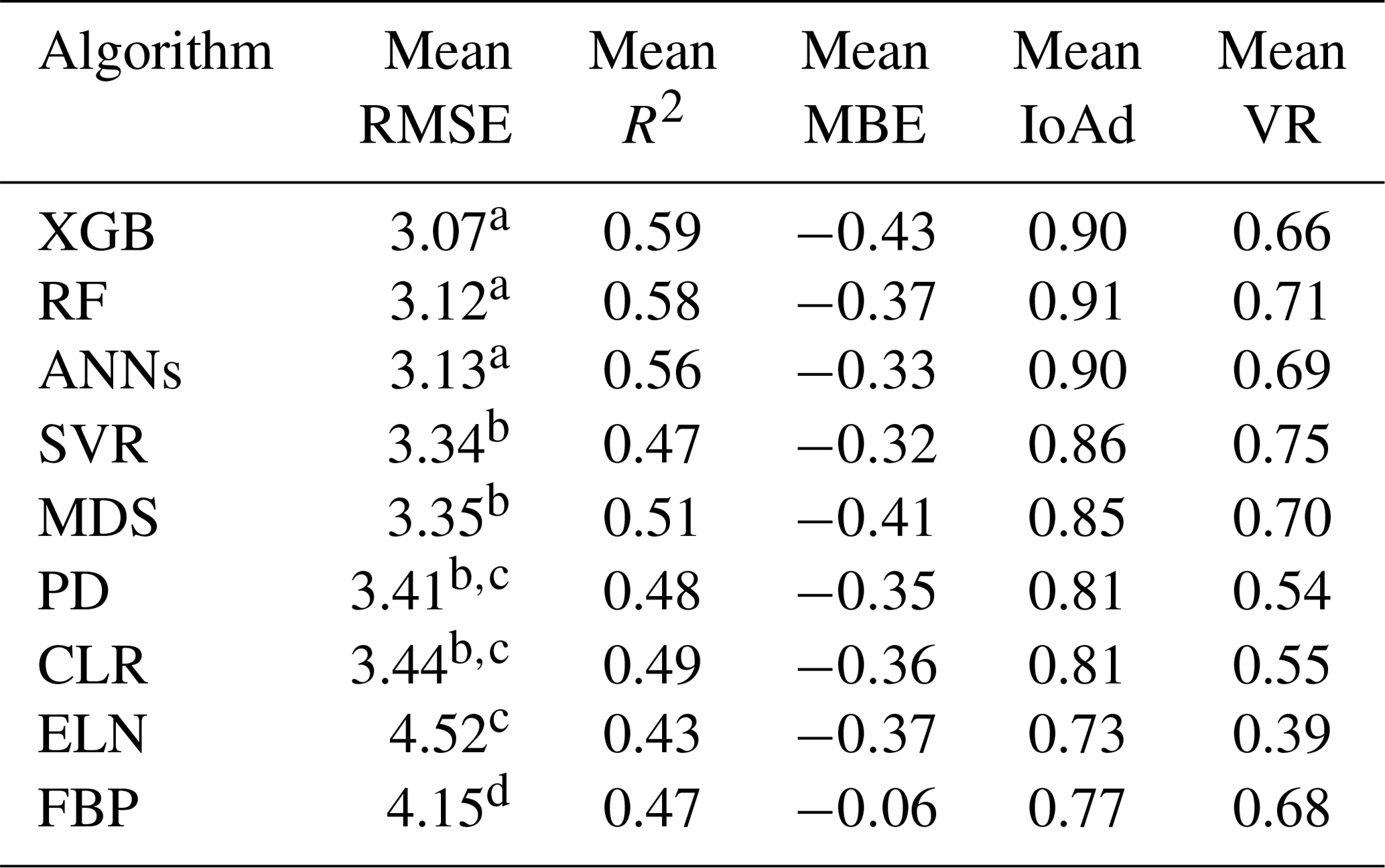
a–d Bonferroni grouping.
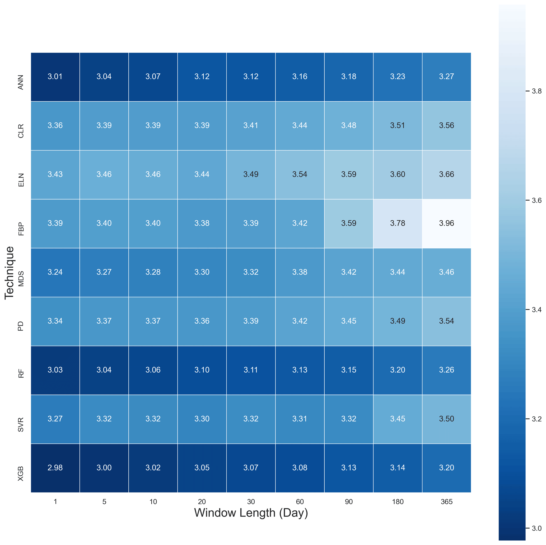
Figure 1A heat map of mean RMSE values of Fc across all sites based on nine algorithms and nine window lengths in 2013.
These outcomes were expected for the XGB as it uses a more regularised model formalisation to control over-fitting (Chen and Guestrin, 2016), which, on paper, leads to better performance against its ML rivals. The relatively poor performance of FBP was also foreseen because, unlike other algorithms, FBP did not use any feature to estimate flux values other than the previous time series of flux values. However, the weaker performance of the ELN compared to CLR was unforeseen as by adding two penalty components to the regression line, the ELN is supposed to improve the long-term prediction compared to the traditional linear regression methods. Tukey's HSD (honestly significant difference) test at the level of 0.05 was applied to the results to determine whether the difference amongst the algorithms was significant (Table 5). When the null hypothesis is confirmed there is no significant difference between the mean values of the RMSE. According to the results, there were significant differences between certain algorithms, and the XGB, RF, and ANNs were different from the rest, showing that these three performed considerably better. Tukey's HSD test, however, did not reject the second error probability between RF, XGB, and ANNs, meaning that the three algorithms were not significantly different from each other. This result agrees with the results of Falge et al. (2001) and Moffat et al. (2007) in the sense that ANNs are one of the best available gap-filling algorithms, and there is no significant difference amongst the appropriate algorithms. However, the test showed that the performance of the MDS was significantly different from the ANNs. It seems that the difference has occurred because of the longer gaps (>10 d) that were absent from previous studies. Finally, it is worth mentioning that Tukey's HSD is well known as a conservative test. That being said, despite no meaningful difference based on Tukey's HSD, XGB and RF might have performed better than ANNs, as the superiority of RF in gap-filling the methane flux over the ANNs, SVR, and MDS has recently been claimed by Kim et al. (2020).
To address this paper's first objective, which was to find the sensitivity of the gap-filling algorithms to the gap window length, we used the averaged RMSE, R2, and MBE for each gap size with the output of all algorithms for all sites (Table 6). The outcome illustrates that the longer the window length got, the larger the RMSE became. Yet, no such pattern was recognisable for the R2 and MBE. As a result, generally, any consecutive gaps longer than 30 d seem to decrease the algorithms' performance noticeably. A reason for this may be that longer windows do not let the algorithms accommodate seasonal changes and therefore different canopy physiological behaviour.
Table 6The average RMSE, R2, and MBE for Fc gap-filling based on the window length, including the outcome of all sites; the differences of RMSE values were tested using the Tukey's HSD test at the level of 0.05.

* means there is not any significant difference between the groups.
According to the MBE values (Table 5), mainly, all algorithms had negative MBEs, indicating an overestimation of the Fc values. This bias varied from tower to tower and depended on the window lengths. For instance, the MBE absolute values were larger in Gingin and Tumbarumba, while they were considerably smaller (closer to zero) at Alice Springs Mulga and Calperum (Supplement). The lower leaf area index of the two latter sites and thus their smaller amounts of photosynthesis are likely to be the reason for this. FBP, nonetheless, provided a substantially lower mean bias (−0.06) compared to the other algorithms, which varied between −0.32 and −0.43.
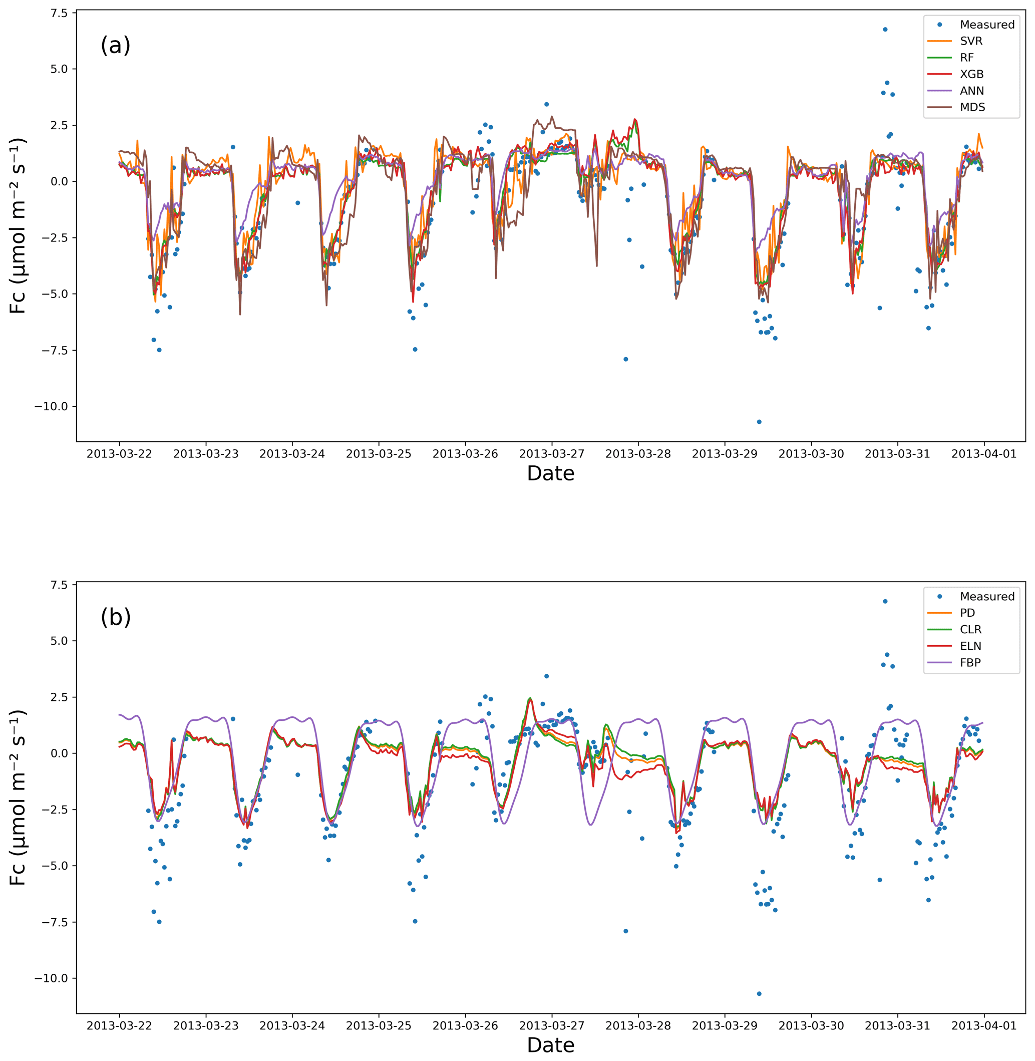
Figure 2Measured vs. estimated values of Fc for Calperum based on a 10 d gap window (22–31 March 2013): (a) the ML algorithm plus the MDS and (b) the linear models plus FBP.
Observations from the EC technique often include extremely low or high values after quality control (QC), especially at night when some of the theoretical assumptions might be violated. One of the practical challenges associated with the EC technique is that it is often difficult to distinguish between the good data and the noise (Aubinet et al., 2012; Burba and Anderson, 2010). This problem seems to affect the outcomes of the gap-filling algorithms in this research, as none of them performed ideally in capturing the observed variance (Table 5). Even though RMSE, R2, and IoAd showed the superiority of the XGB, RF, and ANNs, the variance ratio between the estimated and measured values revealed different information (Table 5), which is recognisable in Fig. 2. The variance ratios (VRs) showed that SVR captured the extreme values of Fc better than the other algorithms, with 0.75 on average. The other ML algorithms (plus the MDS), however, performed similarly with regard to capturing the extremes that match both the expectations and the performance metrics (Table 5).
The linear algorithms, CLR, PD, and ELN, performed worse concerning the VR compared to the ML algorithms, with the VR of Fc for Calperum (Fig. 2) confirming this. Based on the figure, as expected, the ELN performed the worst in capturing the fluctuations in Fc (VR = 0.39), while the performance of the other algorithms, apart from the top five, was not significantly better with the exception of FBP. It is noteworthy that CLR, PD, and ELN frequently predicted nocturnal photosynthesis. Overall, the results showed a significant difference between the top five algorithms (XGB, RF, ANNs, SVR, and MDS) and remaining algorithms, particularly in capturing the fluctuations and the min–max range of Fc. However, a comprehensive comparison shows a slight superiority of the XGB and RF.
3.1.2 Latent heat flux (Fe)
The performance of algorithms for Fe was similar to that for Fc with respect to RMSE, MBE, and R2, as shown in Table 7. This similarity was not surprising since these processes are partially coupled via stomatal conductance (Scanlon and Kustas, 2010; Scanlon and Sahu, 2008). Again, the top three ML algorithms performed better, with XGB and RF being statistically significant as shown by the Tukey's HSD (Table 7). The null hypothesis was not rejected while comparing FBP and SVR, whereas the better performance of the other algorithms was confirmed. As a result, the FBP and SVR provided the most unsatisfactory results in estimating Fe, according to the average values of the RMSE. No significant improvement in RMSE occurred when the gap lengths became shorter than 60 d, meaning that the algorithms' performance did not vary considerably from a 30 d to a 1 d window, especially for the top algorithms (XGB, RF, and ANNs). CLR and PD results were very similar to those for Fc, showing a lower RMSE and higher R2 values against ELN, but the ELN led to a slightly lower MBE. The MBE values also showed moderately high values for the SVR, meaning that there was an absolute bias in its outcome, which might be related to over-fitting. The source of the bias shown by the SVR algorithm (Fig. 3) was its inability to capture the minimum values appropriately, resulting in a considerable overestimation. A common issue in estimating Fe values, which affected all algorithms other than the FBP, was the inability to capture the negative values. In contrast to Fc results, the ANNs did not perform as well as the XGB and RF, which could be due to not capturing the maximum values compared to its rivals.
Table 7The average metrics for Fe gap-filling based on the algorithms, ranked by RMSE using the Tukey's HSD test at the level of 0.05.
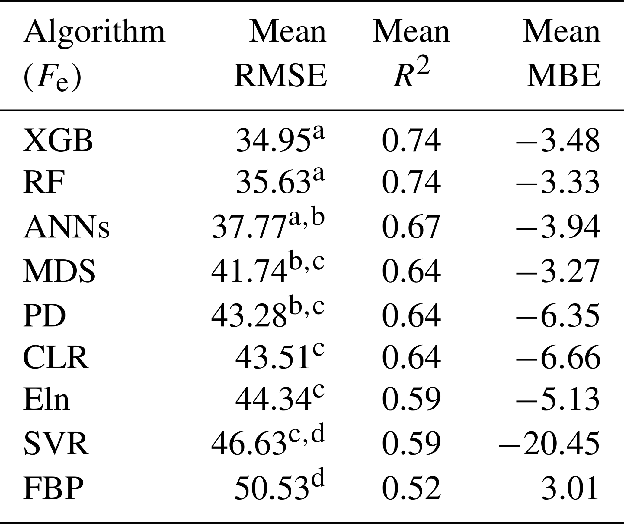
a–d Bonferroni grouping.
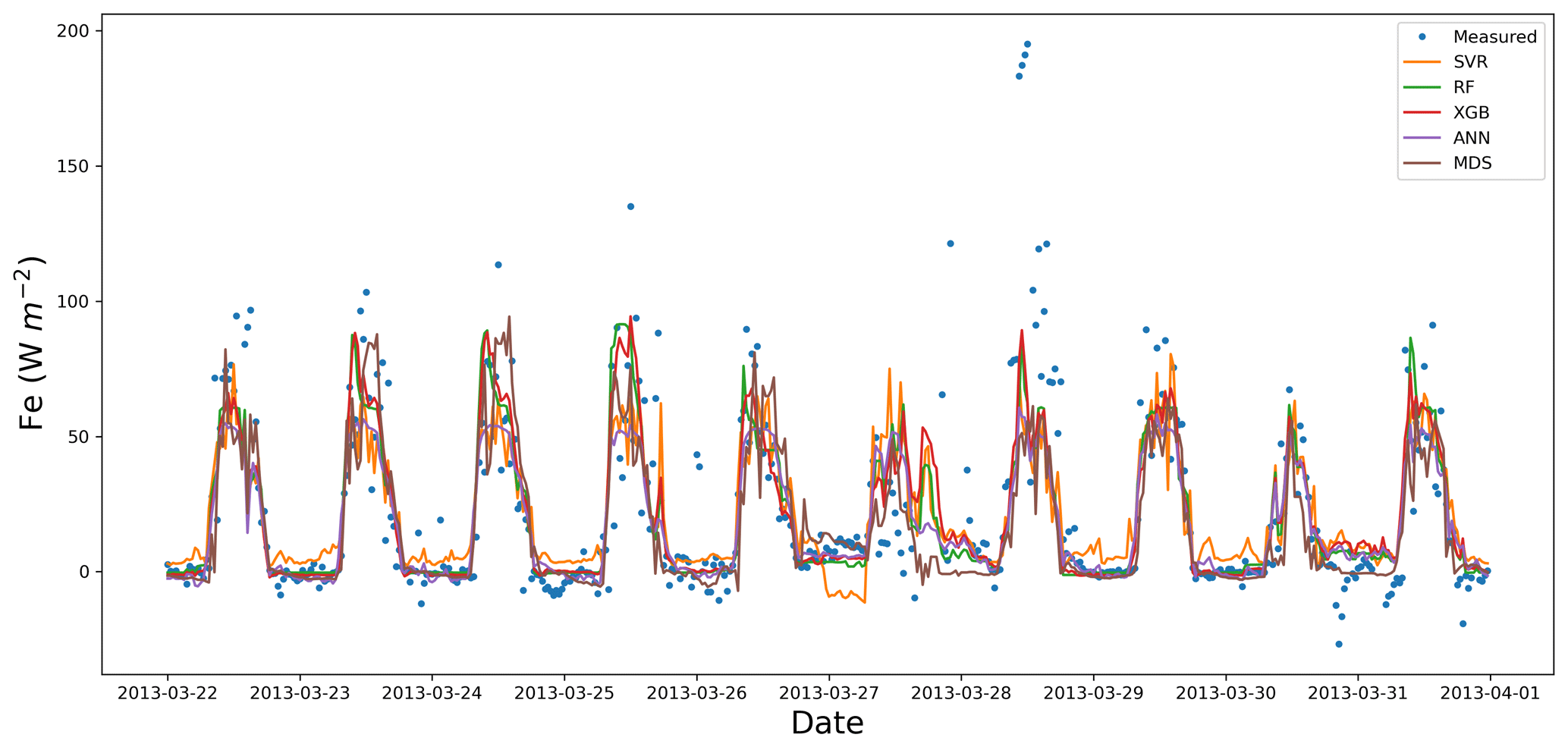
Figure 3Measured vs. estimated values of Fe for Calperum based on a 10 d gap window (22–31 March 2013).
3.1.3 Sensible heat flux (Fh)
As with the other flux results, the metrics of RMSE, R2, and MBE showed slight superiority for XGB and RF, as well as the inferiority of the SVR and FBP to the other algorithms (Table 8). Likewise, the SVR provided relatively large negative values of MBE, showing considerable overestimation. The Tukey's HSD test of the average RMSE values confirmed that the performance of the FBP was significantly different from the rest at the level of 0.05, making FBP the weakest performer for Fh. On the other hand, although there was no significant difference amongst the XGB, RF, and ANNs, the first two were considerably superior over the other algorithms as regards the Tukey's HSD test. Similarly to Fe, estimated values of Fh using SVR had a negative bias (Fig. 4) because it was not able to provide appropriate estimations of Fh minimum values. In contrast, the ANNs performed the best in capturing the minimum values, while the other top algorithms performed almost equally well. Despite the similar performance in capturing the minimum values, ANNs and MDS did not perform as well as XGB and RF in capturing the overall values, resulting in a higher RMSE. Finally, like the other fluxes, the PD performed slightly better than the CLR and ELN.
Table 8The average metrics for Fh gap-filling based on the algorithms, ranked by RMSE using the Tukey's HSD test at the level of 0.05.

a–d Bonferroni grouping.
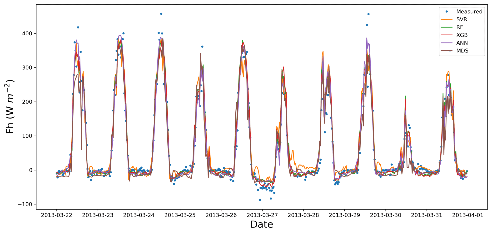
Figure 4Measured vs. estimated values of Fh for Calperum based on a 10 d gap window (22–31 March 2013).
3.2 Meteorological and environmental drivers
Since meteorological and environmental drivers are needed to fill the gaps of the three turbulent fluxes (Fc, Fe, and Fh), the eight algorithms (excluding the MDS) were used to fill these drivers' gaps. The metrics of R2, RMSE, and MBE were calculated for all five towers and nine window lengths (16 meteorological and environmental drivers). Overall, for most meteorological drivers, the linear algorithms, especially the CLR and PD, performed slightly better than the ML algorithms such as the XGB, RF, ANNs, and SVR, except for Ah, Fg, and Fn. This unexpected superiority can be explained based on the following two reasons. Firstly, unlike the fluxes, the input and output features were the same here, e.g. Ta for Ta, which led to solid correlations (e.g. up to 0.99 for atmospheric pressure – ps) as well as strong linear relationships between the independent and dependent features. These strong correlations helped the linear algorithms perform well and reduced ML algorithms' ability to capture the non-linear behaviour of complicated problems. Second, ML algorithms' slight inferiority could be due to data noise; simple linear algorithms such as the CLR are usually relatively less sensitive to noise. Therefore, over-fitting is not an issue for them when the number of observations is big enough (i.e. at least 10 to 20 observations per parameter; Harrell, 2014). The exceptions were Ah, Fn, and Fg, for which values were estimated more accurately by the XGB, ANNs, and RF, especially Fg, with the RMSE of RF and CLR for Fg being 28.91 vs. 33.92, respectively. Tukey's HSD test for the mean RMSE values of Fg confirmed that the XGB, ANNs, and RF showed significantly better results, while, like all other fluxes and drivers, the FBP was the worst algorithm (Table 9). Yet, according to the same test for the other drivers, there was no significant difference between the algorithms other than the FBP, which provided the most significant mean values of the RMSE (results not shown). Importantly, though, none of the algorithms offered adequate estimations for soil moisture (Sws), particularly in drier regions. This weak performance happened because Sws changes dramatically during rainfall in a pulsed manner, often from zero to saturation in a short amount of time, whereas the algorithms had been trained based on the datasets mostly reflecting non-rainy periods. These datasets, consequently, could not fit the algorithms in a way that they could estimate Sws accurately when precipitation occurs and the soil moisture increases dramatically. For instance, in a wet region like Tumbarumba, where the soil faces rainy days frequently, the time series are much less spiky. Thus, the overall performance was better in these regions than the drier ones (e.g. R2 of 0.45 and 0.26 on average for Tumbarumba and Calperum, respectively). In addition, the dataset used to gap-fill the soil moisture was a model derivation from gridded data or regional reanalysis and therefore may not be close to reality. Another challenge of estimating soil moisture comes from the low spatial coherence of soil moisture; it can be extremely different just a couple of hundred metres away due to storms, topography, and soil structure heterogeneity (Reichle et al., 2004; Sahoo et al., 2008).
Table 9The average RMSE for Fg gap-filling based on the algorithms using the Tukey's HSD test at the level of 0.05.

a–d Bonferroni grouping.
Nine gap-filling algorithms were used in this study: eXtreme Gradient Boost (XGB), random forest (RF) algorithm, artificial neural networks (ANNs), marginal distribution sampling (MDS), support vector regression (SVR), classical linear regression (CLR), panel data (PD), elastic net regularisation (ELN), and the Prophet Forecasting Model (FBP). All algorithms performed similarly in estimating the meteorological and environmental drivers (turbulent fluxes included) across all stations except the FBP, which performed poorly because it did not use any ancillary data. The best results were achieved for the 30 d gaps and shorter, while the worst results obtained for the most extended windows of 180 and 365 d. Although most of the algorithms performed almost equally well in estimating meteorological and environmental drivers, the linear algorithms (CLR, ELN, and PD) performed slightly better, though not significantly using Tukey's HSD test. The only apparent exception was Fg, for which the RF provided more accurate and robust estimations. The ML algorithms and MDS, on the other hand, showed their superiority over the linear algorithms while estimating the main fluxes, Fc, Fe, and Fh. For Fc, the XGB, RF, and ANNs performed significantly better than the FBP and all linear algorithms (i.e. the CLR, PD, and ELN, followed closely by the SVR and MDS). The superiority of the ML algorithms and their similar performance agreed with the results of previous researchers (Falge et al., 2001; Moffat et al., 2007), who showed the superiority of non-linear algorithms and no significant difference amongst the top algorithms in estimating Fc. Also, with the slight superiorities of XGB and RF over ANNs, our results confirm that RF performs better for EC flux gap-filling, as noted by Kim et al. (2020) for methane.
The XGB was the most novel ML algorithm used in this research, and based on most performance metrics it provided comparatively robust results in estimating the fluxes. In estimating the meteorological drivers, though, the XGB did not show any superiority over the other algorithms, especially the linear ones. Moreover, the XGB needed 4 to 6 times longer to be trained and tuned, making it a less feasible algorithm when time and processing power are important factors or several years of data need to be gap-filled. Hence, we do not recommend the XGB as an alternative to the current standard algorithms. Nevertheless, because of its local superiorities, this algorithm might be suitable to use in an ensemble model alongside algorithms with different weaknesses.
The RF was the best all-around algorithm amongst the nine algorithms used in this study, providing the best consistent and robust estimates of the fluxes (similar to XGB). It is also less complicated and performs faster than the XGB. The RF also provided the best results for Fg, but the linear algorithms did not perform well. This superiority of RF over ANNs, MDS, and SVR has been shown previously by Kim et al. (2020) for gap-filling of methane, showing that it is worth testing the RF for other towers and fluxes across FLUXNET.
The ANNs estimated the fluxes better than the linear algorithms, most notably for Fc, yet they are not as robust as the XGB and RF in general. For Fc and Fh, the ANNs provided a bias, mainly due to overestimating minimum values when the window lengths were longer than 30 d. However, since the superiority of the XGB and RF was not considerable, it is difficult at this point to suggest using XGB or RF as better alternatives. This is because the utility of ANNs has been validated over a long time in different locations, and they have been considered to be among the most reliable algorithms in the field for more than a decade (Aubinet et al., 2012; Hagen et al., 2006; Kunwor et al., 2017; Moffat et al., 2007). In other words, the superiority of RF should be assessed in several future studies to convince the network to suggest RF instead of ANNs or identify it as another standard gap-filling method. Furthermore, there are a wide variety of different ANN algorithms used in the field (Beringer et al., 2017; Hagen et al., 2006; Isaac et al., 2017; Kunwor et al., 2017; Moffat et al., 2007), and the minor superiority of RF and XGB cannot be generalised without additional case studies. As such, we suggest that other researchers use the RF, especially for Fh and Fc, alongside ANNs to find out which one performs better in challenging scenarios (e.g. when the gaps are long). Another option is to develop ensemble models to improve the results over a single algorithm (Moffat et al., 2007). Ideally, a model with a higher level of flexibility is required in the field (Hagen et al., 2006; Kunwor et al., 2017; Richardson and Hollinger, 2007). Finally, the ANNs, like the other ML algorithms, did not show a consistent superiority over the linear algorithms regarding the environmental drivers. Therefore, we do not recommend using ML algorithms in such scenarios, except for Fg, for which RF seems to be a better option.
The MDS performed similar to, yet not as well as, the XGB, RF, and ANNs in gap-filling the fluxes. Its performance was close to the SVR but was more reliable for Fe and Fh. It is worth mentioning that this performance was achieved despite the MDS using fewer input features. Its performance, however, was comparable with the ML algorithms, particularly when the gap lengths were relatively shorter (equal to or smaller than 10 d). As such, we recommend using the MDS when the gaps are not long or the available input features are limited, especially considering that the MDS performs significantly faster than the ML algorithms and is easier to use.
The SVR showed consistent inferiority to the other ML algorithms and did not fulfil our expectations for the meteorological drivers or for the major fluxes. The only strength of the SVR was that it captured the extreme values better than any other algorithm. However, because of the larger RMSE the mentioned advantage seems to have been achieved suspiciously and might have occurred due to over-fitting. This dubious performance shows that SVR is perhaps more vulnerable to the over-fitting issues regarding these data types. Hence, we suggest the SVR not be used in environmental modelling related to the reviewed drivers and fluxes.
The CLR, the simplest algorithm used in this research, provided a comparatively acceptable performance in estimating the meteorological drivers, except for Fg. This algorithm, however, did not perform well in assessing the fluxes, especially Fc, mainly because of its inability to capture the extreme values caused by the non-linear relation of Fc to its drivers. Overall, considering the CLR's simple, resource-saving, and robust performance for drivers, this algorithm seems to be the most suitable way to fill the gaps of meteorological parameters in similar scenarios in which the same ancillary datasets are available.
The PD performed slightly better than the CLR, yet it did not show a significant superiority over the other linear algorithms used in the research. This unforeseen weak performance can be explained due to a couple of factors. First, one of the assumptions of using the PD is that the cross-sectional behaviour (here towers) is similar under similar conditions (the independent variables), and the only thing that leads to the difference is the specific characteristics of each individual cross section. Contrariwise, it seems that the five towers selected in this research violated this assumption due to their being in widely different ecosystems. Based on previous studies in which the PD performed well (Izady et al., 2013, 2016; Mahabbati et al., 2017), it appears that a decent level of homogeneity is vital for the PD to perform satisfactorily. As in all previous cases, the cross-sectional ecosystem had significant similarities, and the distance between them was smaller. Therefore, the characteristics of cross sections, such as radiation, climate, and rainfall, had considerably more similarity and homogeneity compared with the towers used in this research. Finally, it is worth mentioning that PD has been commonly used to analyse time series with a time resolution of weekly or longer, with some exceptions using daily time steps. In this research, the data resolution was half-hourly instead, which dramatically increased the computational demands of the algorithm and led to days of processing for a single run. This demand happened because the algorithm creates a dummy variable for each time step and the relevant matrix of variables becomes too large to compute with a regular PC. Considering the computational expense of this algorithm, we recommend other researches not use PD when the time resolution is shorter than daily. Despite the limitation, we still encourage further use of PD whenever there is a decent homogeneity level amongst the cross sections and the time resolution is daily or longer.
As a hybrid linear model, the ELN did not show any superiority over the CLR, despite its modifications to provide more accurate estimations. However, ELN performed well in estimating the drivers with slight superiority on some occasions (e.g. for Fld, the CLR is a more proper algorithm to choose for gap-filling the drivers due to its simplicity and lower calculation requirement).
The FBP was a unique algorithm used in this research, as it did not use any independent variables to estimate the values of drivers and fluxes. The FBP performance was the least satisfactory of all the algorithms. Therefore, FBP cannot be considered a reliable alternative for current algorithms to fill gaps, especially longer ones.
Given that some of the environmental drivers that affect Fc are different during the day versus night, separating the diurnal and nocturnal datasets to train the algorithms could improve the outcome. Mainly because of the u* threshold filtering and other problems associated with the nocturnal period, the portion of diurnal data generally far outweighs the nocturnal data portion, which potentially leads to a bias in the algorithm. The same challenge is associated with soil moisture estimation, as the behaviour of the system on sunny days is utterly different from during the rainy periods. Moreover, the system memory and the antecedent conditions are undeniable features associated with soil moisture (Ogle et al., 2015). Therefore, models that can address these considerations are more likely to improve the estimations.
Finally, it is noteworthy that some of the flux drivers used in this study as input features for the gap-filling algorithms are not commonly used or might not globally be available. However, considering that similar relative performance has been achieved in other research for which different sets of input features were used (Kim et al., 2020), the relative performance of the algorithms reviewed in this research should generally provide similar relative performance while using different input features.
Eight different gap-filling algorithms for estimating 16 meteorological drivers and nine algorithms for the three key ecosystem turbulent fluxes (sensible heat flux – Fh, latent heat flux – Fe, and net carbon flux – Fc) were investigated, and their performance was evaluated based on datasets from five towers in Australia. Overall, three ML algorithms, XGB, RF, and ANNs, performed nearly equally well and significantly better than their linear rivals (the CLR, PD, and ELN) in estimating the flux values. However, the linear algorithms performed almost equally well as the ML algorithms in assessing the meteorological drivers. Amongst these nine algorithms, the RF and XGB showed the highest level of robustness and reliability in estimating the Fc, Fe, and Fh. The PD was expected to perform better than the linear methods, and it was hoped that it could compete with the ML algorithms in estimating the fluxes, but it failed to do so. The SVR was the only ML algorithm that did not perform at the same level as the rest of the ML algorithms, which we suspect was due to over-fitting issues, while the MDS performed somewhere in between. Considering the outcomes of previous research undertaken in the OzFlux network (e.g. Cleverly et al., 2013; Isaac et al., 2017), none of the ML algorithms used in this research were proven to provide substantially better flux estimations compared with the standard method (ANNs). Nonetheless, amongst the algorithms tested in this research, the RF showed potential capabilities as an alternative due to its more consistent performance regarding long gaps. Finally, we make suggestions below to improve the results for prospective researchers, as well as the QC and gap-filling procedure for flux networks.
-
Since the RF was more consistent than its competitors, including the ANNs, we suggest it is a good idea to use RF alongside the commonly used algorithms in challenging scenarios, such as with long gaps, to figure out whether this superiority can be generalised.
-
It appears that even after three levels of quality control process by the flux processing software (e.g. PyFluxPro), the data are still quite noisy. These noisy data are an essential source of both uncertainty and inaccuracy of the outcome, regardless of the algorithm used to gap-fill the data. As a result, another level of quality control methods, such as wavelets or matrix factorisation, in addition to the current classical ones used by PyFluxPro and other similar platforms can probably improve the data quality and thereby improve the final imputation results.
-
For future researchers, using recurrent neural networks (RNNs) instead of feed-forward neural networks (FFNNs) could improve estimations. This is likely because RNNs help the model to consider the temporal dynamic behaviour of time series. Unlike FFNNs, wherein the activations flow only from the input layer to the output layer, RNNs also have neuron connections pointing backwards (Géron, 2019). The demand for an algorithm capable of considering time has been mentioned in previous research as one of the reasons why testing new algorithms is needed (Richardson and Hollinger, 2007).
-
Developing ensemble models using algorithms with different weaknesses and strengths may also enhance the results when a single algorithm shows performance deficiency.
All data used in this research are available at this repository address: https://research-repository.uwa.edu.au/en/datasets/a-comparison-of-gap-filling-algorithms-for-eddy-covariance-fluxes (last access: 9 February2018); https://doi.org/10.26182/5f292ee80a0c0 (Mahabbati, 2020).
The supplement related to this article is available online at: https://doi.org/10.5194/gi-10-123-2021-supplement.
The ideas for this study originated in discussions with AM, JB, and ML. AM carried out the analysis, supported by IM and PI. The paper was prepared with contributions from all authors.
The authors declare that they have no conflict of interest.
The authors would like to acknowledge the Terrestrial Ecosystems Research Network (TERN) (https://www.tern.org.au/, last access: 19 August 2019) and the OzFlux network as a part of TERN for supporting the grants and providing the required data, respectively. Atbin Mahabbati also personally thanks Prajwal Kalfe, Caroline Johnson, and Cacilia Ewenz for their support regarding Python programming, English academic writing, and PyFluxPro technical issues.
This paper was edited by Jean Dumoulin and reviewed by Thomas Wutzler and one anonymous referee.
Allison, P. D.: Multiple Imputation for Missing Data: A Cautionary Tale, Sociol. Meth. Res., 28, 301–309, https://doi.org/10.1177/0049124100028003003, 2000.
Altman, D. G. and Bland, J. M.: Missing data, Br. Med. J., 334, 424, https://doi.org/10.1136/bmj.38977.682025.2C, 2007.
Aubinet, M., Grelle, A., Ibrom, A., Rannik, Ü., Moncrieff, J., Foken, T., Kowalski, A. S., Martin, P. H., Berbigier, P., Bernhofer, C., Clement, R., Elbers, J., Granier, A., Grünwald, T., Morgenstern, K., Pilegaard, K., Rebmann, C., Snijders, W., Valentini, R., and Vesala, T.: Estimates of the Annual Net Carbon and Water Exchange of Forests: The EUROFLUX Methodology, Adv. Ecol. Res., 30, 113–175, https://doi.org/10.1016/S0065-2504(08)60018-5, 1999.
Aubinet, M., Vesala, T., and Papale, D.: Eddy Covariance: A Practical Guide to Measurement and Data Analysis, Springer, Dordrecht, the Netherlands, 2012.
Baldocchi, D., Falge, E., Gu, L., Olson, R., Hollinger, D., Running, S., Anthoni, P., Bernhofer, C., Davis, K., Evans, R., Fuentes, J., Goldstein, A., Katul, G., Law, B., Lee, X., Malhi, Y., Meyers, T., Munger, W., Oechel, W., Paw, U. K. T., Pilegaard, K., Schmid, H. P., Valentini, R., Verma, S., Vesala, T., Wilson, K., and Wofsy, S.: FLUXNET: A New Tool to Study the Temporal and Spatial Variability of Ecosystem-Scale Carbon Dioxide, Water Vapor, and Energy Flux Densities, B. Am. Meteorol. Soc., 82, 2415–2434, https://doi.org/10.1175/1520-0477(2001)082<2415:FANTTS>2.3.CO;2, 2001.
Baltagi, B.: Econometric analysis of panel data, available at: http://www.sidalc.net/cgi-bin/wxis.exe/?IsisScript=book2.xis&method=post&formato=2&cantidad=1&expresion=mfn=001143 (last access: 13 March 2018), 1995.
Barr, A. G., Black, T. A., Hogg, E. H., Kljun, N., Morgenstern, K., and Nesic, Z.: Inter-annual variability in the leaf area index of a boreal aspen-hazelnut forest in relation to net ecosystem production, Agr. Forest Meteorol., 126, 237–255, https://doi.org/10.1016/J.AGRFORMET.2004.06.011, 2004.
Barr, A. G., Richardson, A. D., Hollinger, D. Y., Papale, D., Arain, M. A., Black, T. A., Bohrer, G., Dragoni, D., Fischer, M. L., Gu, L., Law, B. E., Margolis, H. A., Mccaughey, J. H., Munger, J. W., Oechel, W., and Schaeffer, K.: Use of change-point detection for friction-velocity threshold evaluation in eddy-covariance studies, Agr. Forest. Meteorol., 171–172, 31–45, https://doi.org/10.1016/j.agrformet.2012.11.023, 2013.
Bennett, N. D., Croke, B. F. W., Guariso, G., Guillaume, J. H. A., Hamilton, S. H., Jakeman, A. J., Marsili-Libelli, S., Newham, L. T. H., Norton, J. P., Perrin, C., Pierce, S. A., Robson, B., Seppelt, R., Voinov, A. A., Fath, B. D., and Andreassian, V.: Characterising performance of environmental models, Environ. Model. Softw., 40, 1–20, https://doi.org/10.1016/j.envsoft.2012.09.011, 2013.
Beringer, J., Hutley, L. B., McHugh, I., Arndt, S. K., Campbell, D., Cleugh, H. A., Cleverly, J., De Dios, V. R., Eamus, D., Evans, B., Ewenz, C., Grace, P., Griebel, A., Haverd, V., Hinko-Najera, N., Huete, A., Isaac, P., Kanniah, K., Leuning, R., Liddell, M. J., MacFarlane, C., Meyer, W., Moore, C., Pendall, E., Phillips, A., Phillips, R. L., Prober, S. M., Restrepo-Coupe, N., Rutledge, S., Schroder, I., Silberstein, R., Southall, P., Sun Yee, M., Tapper, N. J., Van Gorsel, E., Vote, C., Walker, J., and Wardlaw, T.: An introduction to the Australian and New Zealand flux tower network – OzFlux, Biogeosciences, 13, 5895–5916, https://doi.org/10.5194/bg-13-5895-2016, 2016.
Beringer, J., McHugh, I., Hutley, L. B., Isaac, P., and Kljun, N.: Technical note: Dynamic INtegrated Gap-filling and partitioning for OzFlux (DINGO), Biogeosciences, 14, 1457–1460, https://doi.org/10.5194/bg-14-1457-2017, 2017.
Burba, G. and Anderson, D.: A brief practical guide to eddy covariance flux measurements: principles and workflow examples for scientific and industrial applications, available at: https://books.google.com/books?hl=en&lr=&id=mCsI1_8GdrIC&oi=fnd&pg=PA6&dq=A+Brief+Practical+Guide+to+Eddy+Covariance+Flux+Measurements&ots=TKTg25Yq5X&sig=eBYc819N7Jh3gNhJInfEL1e40eM (last access: 11 February 2020), 2010.
Chen, T. and Guestrin, C.: XGBoost: A scalable tree boosting system, in: Proc. ACM SIGKDD Int. Conf. Knowl. Discov. Data Min., 13–17 August 2016, San Francisco, CA, USA, 785–794, https://doi.org/10.1145/2939672.2939785, 2016.
Cleverly, J.: OzFlux data from the Alice Springs Mulga site (AU-ASM), available at: http://data.ozflux.org.au/portal, last access: 9 February 2018.
Cleverly, J., Boulain, N., Villalobos-Vega, R., Grant, N., Faux, R., Wood, C., Cook, P. G., Yu, Q., Leigh, A., and Eamus, D.: Dynamics of component carbon fluxes in a semi-arid Acacia woodland, central Australia, J. Geophys. Res.-Biogeo., 118, 1168–1185, https://doi.org/10.1002/jgrg.20101, 2013.
Devore, J. L.: Probability and Statistics for Engineering and the Sciences., Biometrics, 47, 1638, https://doi.org/10.2307/2532427, 1991.
Dragoni, D., Schmid, H. P., Grimmond, C. S. B., and Loescher, H. W.: Uncertainty of annual net ecosystem productivity estimated using eddy covariance flux measurements, J. Geophys. Res., 112, D17102, https://doi.org/10.1029/2006JD008149, 2007.
Dreyfus, S. E.: Artificial neural networks, back propagation, and the kelley-bryson gradient procedure, J. Guid. Control. Dyn., 13, 926–928, https://doi.org/10.2514/3.25422, 1990.
Drucker, H., Surges, C. J. C., Kaufman, L., Smola, A., and Vapnik, V.: Support vector regression machines, Adv. Neural Inform. Process. Syst., 1, 155–161, 1997.
Falge, E., Baldocchi, D., Olson, R., Anthoni, P., Aubinet, M., Bernhofer, C., Burba, G., Ceulemans, R., Clement, R., Dolman, H., Granier, A., Gross, P., Grünwald, T., Hollinger, D., Jensen, N. O., Katul, G., Keronen, P., Kowalski, A., Lai, C. T., Law, B. E., Meyers, T., Moncrieff, J., Moors, E., Munger, J. W., Pilegaard, K., Rannik, Ü., Rebmann, C., Suyker, A., Tenhunen, J., Tu, K., Verma, S., Vesala, T., Wilson, K., and Wofsy, S.: Gap filling strategies for defensible annual sums of net ecosystem exchange, Agr. Forest Meteorol., 107, 43–69, https://doi.org/10.1016/S0168-1923(00)00225-2, 2001.
Farley, B. G. and Clark, W. A.: Simulation of self-organizing systems by digital computer, IRE Prof. Gr. Inf. Theory, 4, 76–84, https://doi.org/10.1109/TIT.1954.1057468, 1954.
Freedman, D. A.: Statistical Models: Theory and Practice, 2nd Edn., Cambridge University Press, available at: https://www.cambridge.org/au/academic/subjects/statistics-probability/statistical-theory-and-methods/statistical-models-theory-and-practice-2nd-edition?format=PB (last access: 21 March 2020), 2009.
Friedman, J. H.: Greedy Function Approximation: A Gradient Boosting Machine on JSTOR, Ann. Stat., 29, 1189–1232, 2001.
Friedman, J. H.: Stochastic gradient boosting, Comput. Stat. Data Anal., 38, 367–378, https://doi.org/10.1016/S0167-9473(01)00065-2, 2002.
Gani, A., Mohammadi, K., Shamshirband, S., Altameem, T. A., Petković, D., and Ch, S.: A combined method to estimate wind speed distribution based on integrating the support vector machine with firefly algorithm, Environ. Prog. Sustain. Energ., 35, 867–875, https://doi.org/10.1002/ep.12262, 2016.
Géron, A.: Hands-on machine learning with Scikit-Learn and TensorFlow: concepts, tools, and techniques to build intelligent systems, available at: https://books.google.com.au/books?hl=en&lr=&id=HHetDwAAQBAJ&oi=fnd&pg=PP1&dq=hands-on+machine+learning+with+&ots=0KvfZqlgOo&sig=5tH2IHRsUaTMTy6CfQ6lw3UDKa4 (last access: 7 February 2020), 2019.
Hagen, S. C., Braswell, B. H., Linder, E., Frolking, S., Richardson, A. D., and Hollinger, D. Y.: Statistical uncertainty of eddy flux – Based estimates of gross ecosystem carbon exchange at Howland Forest, Maine, J. Geophys. Res.-Atmos., 111, 1–12, https://doi.org/10.1029/2005JD006154, 2006.
Harrell, F. E.: Regression Modeling Strategies: With Applications to Linear Models, Logistic, available at: https://books.google.com.au/books?hl=en&lr=&id=94RgCgAAQBAJ&oi=fnd&pg=PR7&dq=regression+modeling+strategies+frank+harrell&ots=ZAt4RsaS1r&sig=mikE1s9G4IXzqZKEie-iVA9GTV0&redir_esc=y#v=onepage&q=regression modeling strategies frankharrell&f=false (last access: 11 February 2020), 2014.
Harvey, A. C. and Peters, S.: Estimation procedures for structural time series models, J. Forecast., 9, 89–108, https://doi.org/10.1002/for.3980090203, 1990.
Haverd, V., Briggs, P., Trudinger, C., Nieradzik, L., and Canadell, P.: BIOS2 – Frontier Modelling of the Australian Carbon and Water Cycles, CSIRO, Hobart, Tasmania, Australia, 2015.
Ho, T. K.: Random decision forests, in: Proc. Int. Conf. Doc. Anal. Recognition, ICDAR, 14–16 August 1995, Montreal, QC, Canada, 278–282, https://doi.org/10.1109/ICDAR.1995.598994, 1995.
Ho, T. K.: The Random Subspace Method for Constructing Decision Forests, IEEE T. Pattern Anal. Mac. Intel., 20, 832–844, 1998.
Hollinger, D. Y., Goltz, S. M., Davidson, E. A., Lee, J. T., Tu, K., and Valentine, H. T.: Seasonal patterns and environmental control of carbon dioxide and water vapour exchange in an ecotonal boreal forest, Global Change Biol., 5, 891–902, https://doi.org/10.1046/j.1365-2486.1999.00281.x, 1999.
Hsiao, C., Hashem Pesaran, M., and Kamil Tahmiscioglu, A.: Maximum likelihood estimation of fixed effects dynamic panel data models covering short time periods, J. Econom., 109, 107–150, https://doi.org/10.1016/S0304-4076(01)00143-9, 2002.
Hui, D., Wan, S., Su, B., Katul, G., Monson, R., and Luo, Y.: Gap-filling missing data in eddy covariance measurements using multiple imputation (MI) for annual estimations, Agr. Forest Meteorol., 121, 93–111, https://doi.org/10.1016/S0168-1923(03)00158-8, 2004.
Hutley, L. B., Leuning, R., Beringer, J., and Cleugh, H. A.: The utility of the eddy covariance technique as a tool in carbon accounting: tropical savanna as a case study, Aust. J. Bot., 53, 663–675, 2005.
Isaac, P., Cleverly, J., McHugh, I., Van Gorsel, E., Ewenz, C., and Beringer, J.: OzFlux data: Network integration from collection to curation, Biogeosciences, 14, 2903–2928, https://doi.org/10.5194/bg-14-2903-2017, 2017.
Izady, A., Davary, K., Alizadeh, A., Moghaddam Nia, A., Ziaei, A. N., and Hasheminia, S. M.: Application of NN-ARX Model to Predict Groundwater Levels in the Neishaboor Plain, Iran, Water Resour. Manage., 27, 4773–4794, https://doi.org/10.1007/s11269-013-0432-y, 2013.
Izady, A., Abdalla, O., and Mahabbati, A.: Dynamic panel-data-based groundwater level prediction and decomposition in an arid hardrock–alluvium aquifer, Environ. Earth Sci., 75, 1–13, https://doi.org/10.1007/s12665-016-6059-6, 2016.
Kang, H.: The prevention and handling of the missing data, Korean J. Anesthesiol., 64, 402–406, https://doi.org/10.4097/kjae.2013.64.5.402, 2013.
Kim, Y., Johnson, M. S., Knox, S. H., Black, T. A., Dalmagro, H. J., Kang, M., Kim, J., and Baldocchi, D.: Gap-filling approaches for eddy covariance methane fluxes: A comparison of three machine learning algorithms and a traditional method with principal component analysis, Global Change Biol., 26, 1499–1518, https://doi.org/10.1111/gcb.14845, 2020.
Kock, N. and Gaskins, L.: Simpson's paradox, moderation and the emergence of quadratic relationships in path models: an information systems illustration, Int. J. Appl. Nonlin. Sci., 2, 200–234, https://doi.org/10.1504/ijans.2016.077025, 2016.
Kunwor, S., Starr, G., Loescher, H. W., and Staudhammer, C. L.: Preserving the variance in imputed eddy-covariance measurements: Alternative methods for defensible gap filling, Agr. Forest Meteorol., 232, 635–649, https://doi.org/10.1016/j.agrformet.2016.10.018, 2017.
Law, B. E., Falge, E., Gu, L., Baldocchi, D. D., Bakwin, P., Berbigier, P., Davis, K., Dolman, A. J., Falk, M., Fuentes, J. D., Goldstein, A., Granier, A., Grelle, A., Hollinger, D., Janssens, I. A., Jarvis, P., Jensen, N. O., Katul, G., Mahli, Y., Matteucci, G., Meyers, T., Monson, R., Munger, W., Oechel, W., Olson, R., Pilegaard, K., Paw U H, K. T., Thorgeirsson, H., Valentini, R., Verma, S., Vesala, T., Wilson, K., and Wofsy, S.: Jourassess2, Agr. Forest Meteorol., 113, 97–120, 2002.
Lee, X., Fuentes, J. D., Staebler, R. M., and Neumann, H. H.: Long-term observation of the atmospheric exchange of CO2 with a temperate deciduous forest in southern Ontario, Canada, J. Geophys. Res.-Atmos., 104, 15975–15984, https://doi.org/10.1029/1999JD900227, 1999.
Little, R. J. A.: Statistical analysis with missing data, 2nd Edn., edited by: Rubin, D. B., Wiley, Hoboken, NJ, 2002.
Mahabbati, A. (Creator): A comparison of gap-filling algorithms for eddy covariance fluxes and their drivers, The University of Western Australia, AliceSpringsMulga_AWS(.nc), AliceSpringsMulga_BIOS2(.nc), AliceSpringsMulga_ACCESS(.nc), AliceSpringsMulga_L3(.nc), AliceSpringsMulga_L4(.nc), Calperum_AWS(.nc), Calperum_BIOS2(.nc), Calperum_L3(.nc), Calperum_L4(.nc), Calperum_ACCESS(.nc), Gingin_AWS(.nc), Gingin_ACCESS(.nc), Gingin_BIOS2(.nc), Gingin_L3(.nc), Gingin_L4(.nc), HowardSprings_AWS(.nc), HowardSprings_BIOS2(.nc), HowardSprings_ACCESS(.nc), HowardSprings_L4(.nc), Tumbarumba_ACCESS(.nc), HowardSprings_L3(.nc), Tumbarumba_BIOS2(.nc), Tumbarumba_L3(.nc), Tumbarumba_L4(.nc), Tumbarumba_AWS(.nc), https://doi.org/10.26182/5f292ee80a0c0, 2020.
Mahabbati, A., Izady, A., Mousavi Baygi, M., Davary, K., and Hasheminia, S. M.: Daily soil temperature modeling using `panel-data' concept, J. Appl. Stat., 44, 1385–1401, https://doi.org/10.1080/02664763.2016.1214240, 2017.
Menzer, O., Moffat, A. M., Meiring, W., Lasslop, G., Schukat-Talamazzini, E. G., and Reichstein, M.: Random errors in carbon and water vapor fluxes assessed with Gaussian Processes, Agr. Forest Meteorol., 178–179, 161–172, https://doi.org/10.1016/j.agrformet.2013.04.024, 2013.
Moffat, A. M., Papale, D., Reichstein, M., Hollinger, D. Y., Richardson, A. D., Barr, A. G., Beckstein, C., Braswell, B. H., Churkina, G., Desai, A. R., Falge, E., Gove, J. H., Heimann, M., Hui, D., Jarvis, A. J., Kattge, J., Noormets, A., and Stauch, V. J.: Comprehensive comparison of gap-filling techniques for eddy covariance net carbon fluxes, Agr. Forest Meteorol., 147, 209–232, https://doi.org/10.1016/j.agrformet.2007.08.011, 2007.
Molenberghs, G., Fitzmaurice, G., Kenward, M. G., Tsiatis, A., Verbeke, G., Fitzmaurice, G., Kenward, M. G., Tsiatis, A., and Verbeke, G.: Handbook of Missing Data Methodology, Chapman and Hall/CRC, Boca Raton, Florida, 2014.
Ogle, K., Barber, J. J., Barron-Gafford, G. A., Bentley, L. P., Young, J. M., Huxman, T. E., Loik, M. E., and Tissue, D. T.: Quantifying ecological memory in plant and ecosystem processes, Ecol. Lett., 18, 221–235, https://doi.org/10.1111/ele.12399, 2015.
Papale, D. and Valentini, R.: A new assessment of European forests carbon exchanges by eddy fluxes and artificial neural network spatialization, Global Change Biol., 9, 525–535, https://doi.org/10.1046/j.1365-2486.2003.00609.x, 2003.
Pilegaard, K., Hummelshøj, P., Jensen, N. O., and Chen, Z.: Two years of continuous CO2 eddy-flux measurements over a Danish beech forest, Agr. Forest Meteorol., 107, 29–41, https://doi.org/10.1016/S0168-1923(00)00227-6, 2001.
Reichle, R. H., Koster, R. D., Dong, J., and Berg, A. A.: Global soil moisture from satellite observations, land surface models, and ground data: Implications for data assimilation, J. Hydrometeorol., 5, 430–442, https://doi.org/10.1175/1525-7541(2004)005<0430:GSMFSO>2.0.CO;2, 2004.
Reichstein, M., Falge, E., Baldocchi, D., Papale, D., Aubinet, M., Berbigier, P., Bernhofer, C., Buchmann, N., Gilmanov, T., Granier, A., Grünwald, T., Havránková, K., Ilvesniemi, H., Janous, D., Knohl, A., Laurila, T., Lohila, A., Loustau, D., Matteucci, G., Meyers, T., Miglietta, F., Ourcival, J. M., Pumpanen, J., Rambal, S., Rotenberg, E., Sanz, M., Tenhunen, J., Seufert, G., Vaccari, F., Vesala, T., Yakir, D., and Valentini, R.: On the separation of net ecosystem exchange into assimilation and ecosystem respiration: Review and improved algorithm, Global Change Biol., 11, 1424–1439, https://doi.org/10.1111/j.1365-2486.2005.001002.x, 2005.
Richardson, A. D. and Hollinger, D. Y.: A method to estimate the additional uncertainty in gap-filled NEE resulting from long gaps in the CO2 flux record, Agr. Forest Meteorol., 147, 199–208, https://doi.org/10.1016/j.agrformet.2007.06.004, 2007.
Richardson, A. D., Braswell, B. H., Hollinger, D. Y., Burman, P., Davidson, E. A., Evans, R. S., Flanagan, L. B., Munger, J. W., Savage, K., Urbanski, S. P., and Wofsy, S. C.: Comparing simple respiration models for eddy flux and dynamic chamber data, Agr. Forest Meteorol., 141, 219–234, https://doi.org/10.1016/J.AGRFORMET.2006.10.010, 2006.
Richardson, A. D., Aubinet, M., Barr, A. G., Hollinger, D. Y., Ibrom, A., Lasslop, G., and Reichstein, M.: Uncertainty Quantification, in: Eddy Covariance, Springer, Dordrecht, the Netherlands, 173–209, 2012.
Sahoo, A. K., Dirmeyer, P. A., Houser, P. R., and Kafatos, M.: A study of land surface processes using land surface models over the Little River Experimental Watershed, Georgia, J. Geophys. Res.-Atmos., 113, D20121, https://doi.org/10.1029/2007JD009671, 2008.
Scanlon, T. M. and Kustas, W. P.: Partitioning carbon dioxide and water vapor fluxes using correlation analysis, Agr. Forest Meteorol., 150, 89–99, https://doi.org/10.1016/j.agrformet.2009.09.005, 2010.
Scanlon, T. M. and Sahu, P.: On the correlation structure of water vapor and carbon dioxide in the atmospheric surface layer: A basis for flux partitioning, Water Resour. Res., 44, W10418, https://doi.org/10.1029/2008WR006932, 2008.
Staebler, M.: Long-term observation of the atmospheric exchange of CO2 with a temperate deciduous forest in southern Ontario, Canada ecosystem net ecosystem production turbulence is turbulent, Data Process, 104, 975–984, 1999.
Tannenbaum, C. E.: The empirical nature and statistical treatment of missing data., Diss. Abstr. Int. Sect. A Humanit. Soc. Sci., available at: http://ovidsp.ovid.com/ovidweb.cgi?T=JS&PAGE=reference&D=psyc7&NEWS=N&AN=$2010-99071-044 (last access: 20 February 2018), 2010.
Taylor, S. J. and Letham, B.: Forecasting at Scale, Am. Stat., 72, 37–45, https://doi.org/10.1080/00031305.2017.1380080, 2018.
Tenhunen, J. D., Valentini, R., Köstner, B., Zimmermann, R., and Granier, A.: Variation in forest gas exchange at landscape to continental scales, Ann. Sci. For., 55, 1–11, https://doi.org/10.1051/forest:19980101, 1998.
Wooldridge, J. M.: Econometric Analysis of Cross Section and Panel Data, MIT Press, Cambridge, 2002.
Ye, J., Chow, J.-H., Chen, J., and Zheng, Z.: Stochastic gradient boosted distributed decision trees, in: Proceeding of the 18th ACM conference on Information and knowledge management – CIKM'09, ACM Press, New York, USA, p. 2061, 2009.
Zhao, X. and Huang, Y.: A comparison of three gap filling techniques for eddy covariance net carbon fluxes in short vegetation ecosystems, Adv. Meteorol., 2015, 1–12, https://doi.org/10.1155/2015/260580, 2015.
Zou, H. and Hastie, T.: Regularization and variable selection via the elastic net, available at: https://citeseerx.ist.psu.edu/viewdoc/download;jsessionid=22250F01CC77D55C54B6BAFF4512C9E3?doi=10.1.1.124.4696&rep=rep1&type=pdf (last access: 28 August 2019), 2005.