The fluxgate magnetometer of the Low Orbit Pearl Satellites (LOPS): overview of in-flight performance and initial results

The Low Orbit Pearl Satellite series consists of six constellations, with each constellation consisting of three identical microsatellites that line up just like a string of pearls. The first constellation of three satellites were launched on 29 September 2017, with an inclination of ∼ 35.5^∘ and ∼ 600 km altitude. Each satellite is equipped with three identical fluxgate magnetometers that measure the in situ magnetic field and its low-frequency fluctuations in the Earth's low-altitude orbit. The triple sensor configuration enables separation of stray field effects generated by the spacecraft from the ambient magnetic field (e.g., Zhang et al., 2006). This paper gives a general description of the magnetometer including the instrument design, calibration before launch, in-flight calibration, in-flight performance, and initial results. Unprecedented spatial coverage resolution of the magnetic field measurements allow for the investigation of the dynamic processes and electric currents of the ionosphere and magnetosphere, especially for the ring current and equatorial electrojet during both quiet geomagnetic conditions and storms. Magnetic field measurements from LOPS could be important for studying the method to separate their contributions of the Magnetosphere-Ionosphere (M-I) current system.

1 Introduction

Magnetic fields are fundamental elements in characterizing the Earth's environment. Accurate and high spatial coverage of the magnetic field vector measurements along the orbits (35.5^∘ inclination, 600 km altitude) of the Low Orbit Pearl Satellites (LOPS) allow for separation of temporal and spatial variations of the magnetic field and hence are beneficial to study the magnetospheric and ionospheric magnetic features of the external field at mid- to low latitude, which is important for establishing a high-precision geomagnetic model (e.g., Hulot et al., 2015; Olsen et al., 2016). In particular, with the simultaneous multiple magnetic field observations at mid- to low latitude, the ring current, especially the partial ring current, as well as the equatorial electrojet (EEJ) at different local times could be studied in great detail. In addition, the dynamic change of the South Atlantic Anomaly under different geomagnetic activities could also be monitored with the help of dense magnetic field observation coverage of local time at mid- to low latitude.

The magnetic field intensity at low Earth orbit is in the range of ∼ 20 000 to ∼ 60 000 nT. In addition, some scientific research of the physical processes such as the geomagnetic pulsations require a magnetic field resolution as high as 0.1 nT (e.g., Sutcliffe et al., 2000). These conditions raise high requirements for the low Earth orbit magnetic measurements such as satellite platforms, instrumentation design, and data calibration. There were no global high-precision measurements of the Earth's magnetic field until the launch of the OGO-2 satellite in 1965, though this satellite only measured the magnetic intensity at altitudes from 400 to 1510 km (Cain and Langel, 1971). The MAGSAT was the first global magnetic vector survey satellite, which operated for about 6 months from November 1979 to April 1980 (Mobley et al., 1980). It was about 20 years after the MAGSAT mission that the more recent and high-precision global magnetic satellite observations became available: the ørsted satellite (Olsen, 2007), CHAMP (Maus, 2007), and SAC-C (Stauning, 2002) carried nearly the same instrumentation and provided over a decade of unique geomagnetic data sets, which were used for establishing a lot of geomagnetic models (e.g., Olsen, 2002, Olsen et al., 2003, 2010; Sabaka et al., 2004, 2015; Maus et al., 2007; Finlay et al., 2016). The European Space Agency (ESA) three-satellites mission SWARM, launched on 22 November 2013, provided not only the global magnetic field measurements but also the east–west gradient of the magnetic field with the help of two spacecraft flying side by side with a separation in longitude of about 1.4^∘ (Friis-Christensen et al., 2006). The SWARM mission provides the best survey of the geomagnetic field and its spatial and temporal evolution. During the past few decades, the academic–commercial consortium provided magnetic field data from the Iridium constellation of more than 70 communication satellites to the geospace science community. Although without magnetic cleanliness, the iridium engineering magnetometer data also provided important information for studying and sensing the global field-aligned current (Anderson et al., 2000, 2002, Waters et al., 2001; Anderson et al., 2008). Using multipoint magnetic measurements, the magnetic measurements from the three Space Technology 5 (ST5) satellites (Slavin et al., 2008; Le et al. (2009)) for the first time separated the temporal and spatial variations in field-aligned current perturbations in low Earth orbit on timescales of ∼ 10 s to 10 min. There are three identical fluxgate magnetometers on the LOPS, with sensors 1 and 3 mounted at the tips of two 1.5 m booms on each side of the spacecraft, as shown in Fig. 1. Sensor 2 is mounted at the middle of boom on the sensor 3 side. Without magnetic cleaning of the satellite platform, the high-precision geomagnetic measurements could not be performed before in-flight calibration. Previous studies have shown that the spacecraft stray field caused by magnetic material or generated by the platform currents could be detected and removed below the threshold of the scientific requirement using a difference or gradient method based on dual-sensor measurements (e.g., Zhang et al., 2006, 2008; Auster et al., 2008; Ludlam et al., 2008; Pope et al., 2011). With three sensors on the LOPS, separation of the ambient and stray magnetic fields (both DC and AC field) becomes possible. The magnetic investigation of the spacecraft body, the payloads, and the solar panels were carefully examined before the launch of each satellite. In addition, in-flight stray field determination is carried out based on several different methods. We will give a detailed description of the stray field corrections for both pre- and in-flight periods in Sect. 4.2.

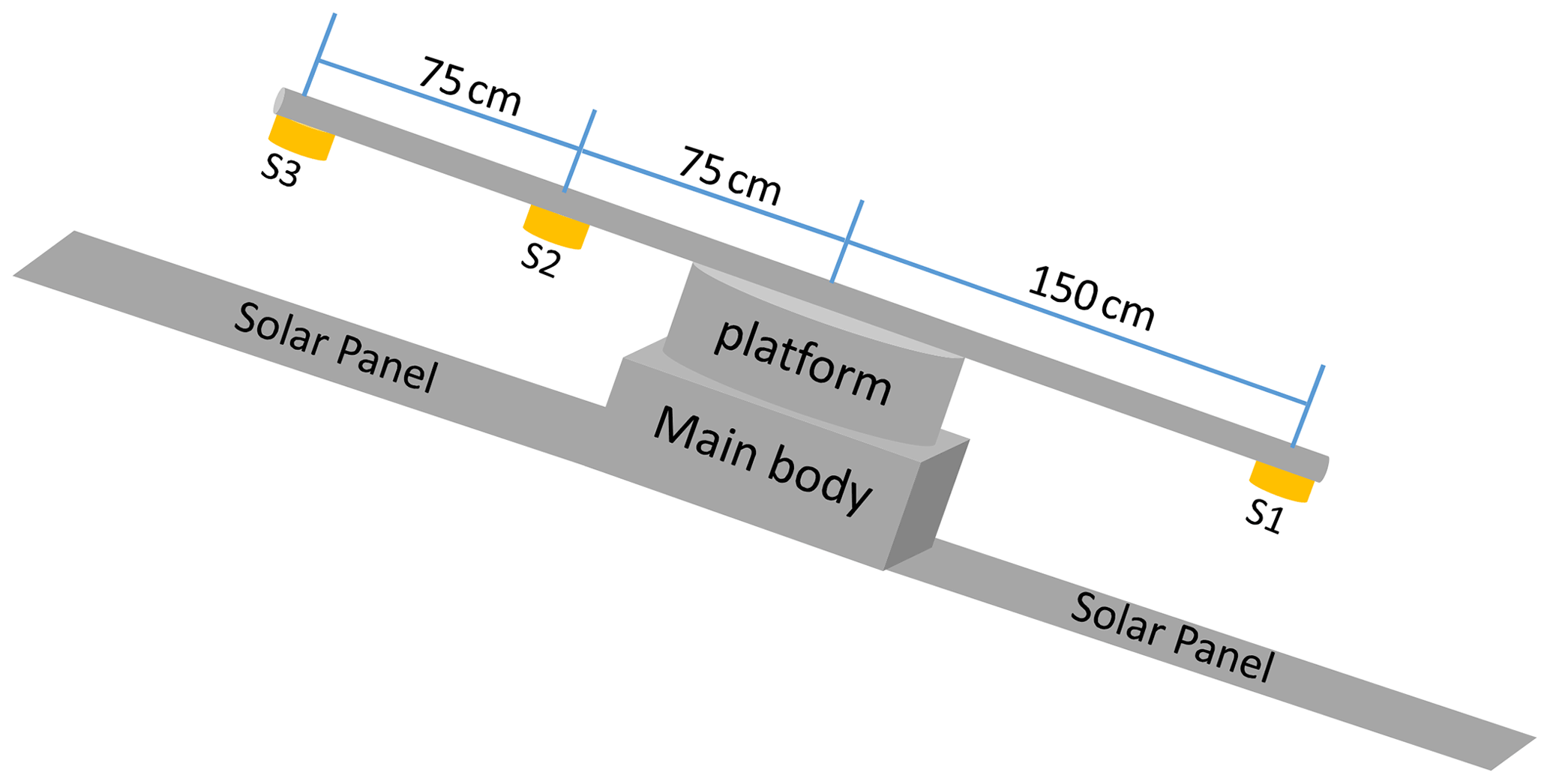
Figure 1 Schematic diagram of the installation positions of the three magnetometer sensors on board the satellite.

The Star Imager (SIM), which determines the attitude of the satellite with high accuracy, is mounted in the satellite body. This configuration will lead to time variation of the three Euler angles (which describe the rotation between the coordinate system of the magnetometer and the SIM) to some extent due to the fact that the boom, which connects the magnetometer and the satellite body, is not totally rigid and it will vibrate in orbit (Olsen et al., 2003).

The rest of this paper is organized as follows. In Sect. 2 we give the magnetometer instrument description, which includes the fluxgate sensor and the sensor electronics. The magnetometer calibration for both pre- and in-flight magnetometer calibration is the main topic of Sect. 3. In Sect. 4, we give the initial scientific results. A summary is given in Sect. 5.

2 Instrument description

2.1 Overview

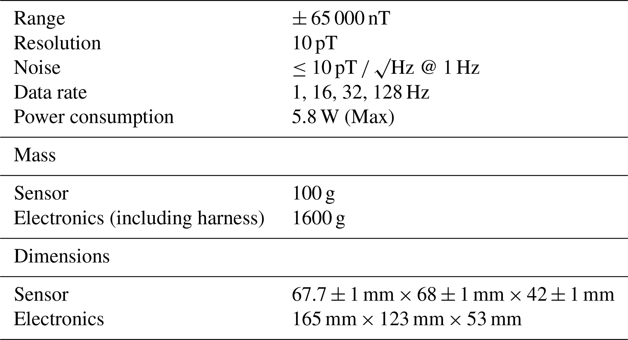
The fluxgate magnetometers are the most common magnetometers used for space magnetic field measurements. The LOPS flux magnetometer consists of a vector-compensated three-axis fluxgate sensor unit and a digital electronics unit on a single printed circuit board. The electronic box comprises three sensor electronics boards, the data processing unit (DPU) board, and a power control unit. Both the sensors and electronic on board the LOPS benefit from the heritage of the magnetometer on board the Venus Express (Zhang et al., 2006) and the THEMIS (Auster et al., 2008). The main instrument parameters are listed in Table 1.

Table 1 The instrument parameters of the magnetometers on board the LOPS.

2.2 Fluxgate sensors

The fluxgate sensor consists of a sense coil surrounding an inner excitation coil that is closely wound around highly permeable, low-noise magnetic ring cores with good offset stability. The material used for the magnetic ring cores is similar to that used in the magnetometer on-board the Venus Express (Zhang et al., 2006) and Equator-S and has been tested for a strict procedure.

The sense coil consists of three mutually perpendicular component coils and has a triaxial concentric shape in order to make sure the three measured components are the magnetic information from a spatial location with different directions.

The feedback coil is also composed of three mutually perpendicular coils. The feedback circuit generates additional three-component magnetic fields in real time in order to ensure the uniformity and stability of the generated magnetic field; each direction coil is composed of two sets of parallel coils.

A continuous repeating cycle electromagnetic signal driven by the excitation coil is monitored by the sense coil with the principal frequency twice that of the excitation signal frequency and whose strength and phase orientation vary directly with the external field magnitude and polarity.

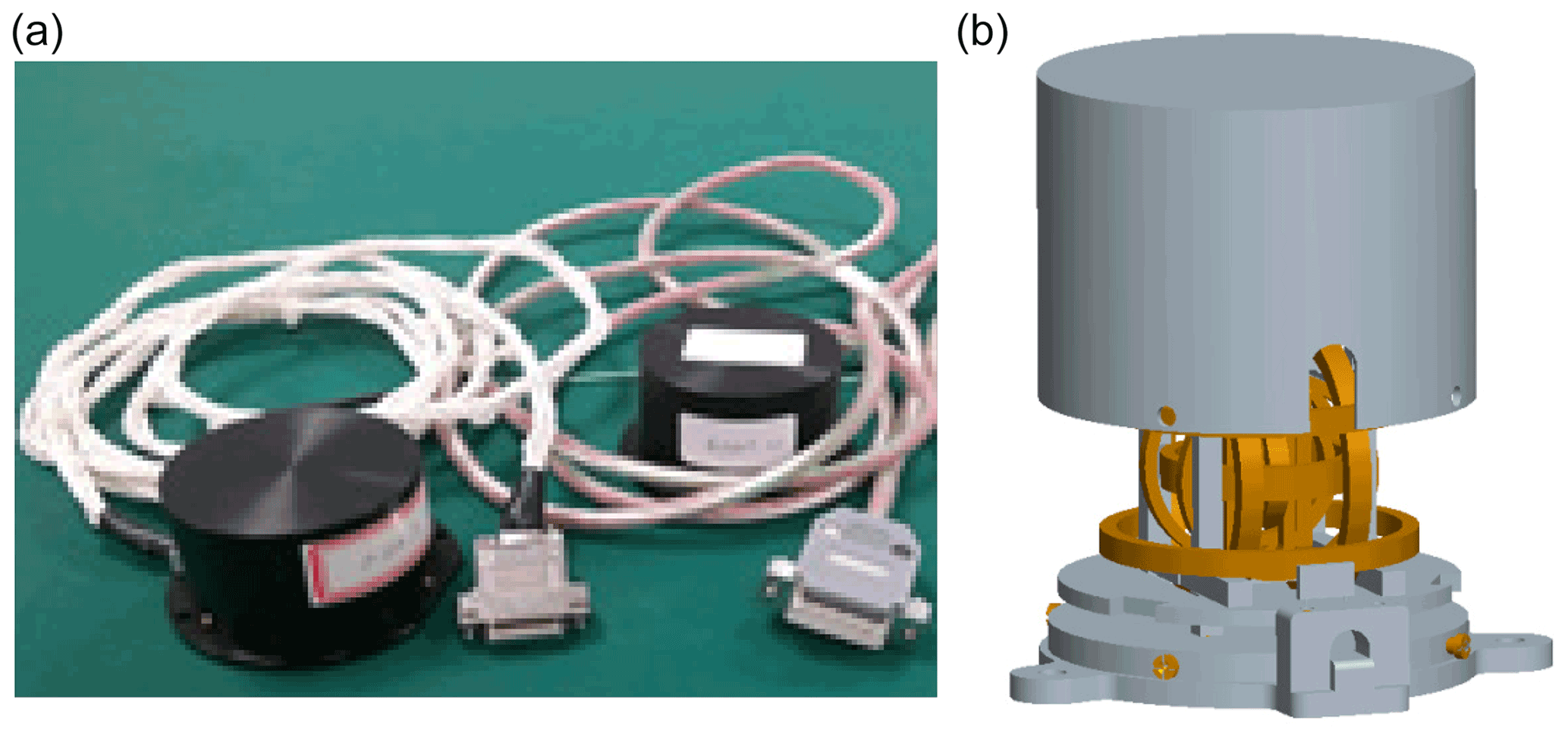
The sensor photograph and the structure design diagram are shown in Fig. 2a and b.

Figure 2 A real sensor picture (a) and structure design diagram of the sensor (b).

2.3 Sensor electronics

The sensor electronics consists of excitation module circuitry, sense signal acquisition module circuitry, feedback module circuitry, and temperature module circuitry. The excitation module, which is composed of the excitation signal portion generated in the FPGA and MOS drive amplification circuit, is used to generate the excitation signal required for the excitation coil. The schematic of the excitation module circuit is shown in Fig. 3.

Figure 3 The schematic of the excitation module circuit.

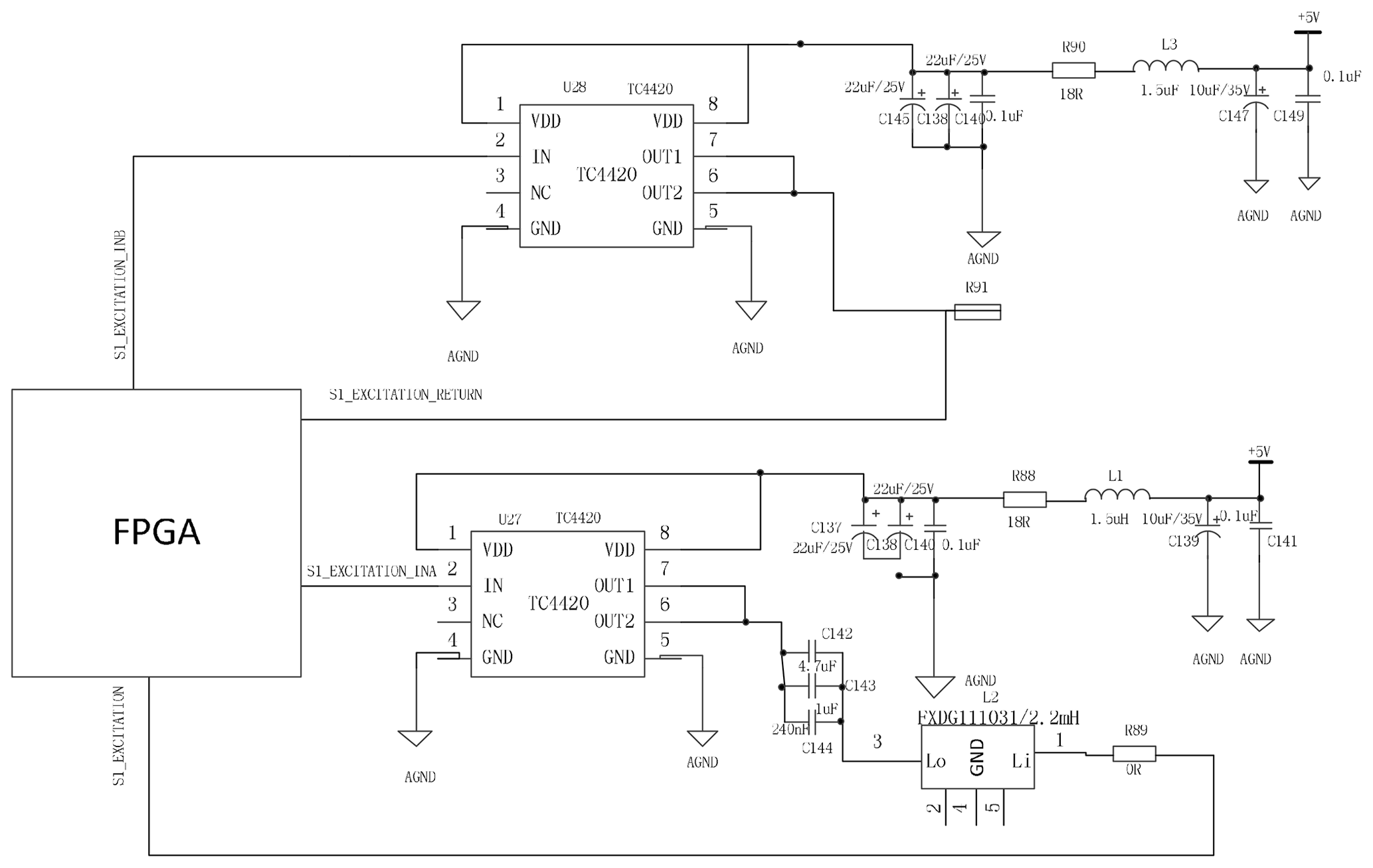
In the excitation module circuitry, the FPGA generates two 9.6 kHz square wave signals with opposite phases that are amplified by the power amplifier circuit and transmitted to the excitation coil. In addition, the excitation circuit also includes a circuit that forms LC resonance with the internal excitation coil of the probe.

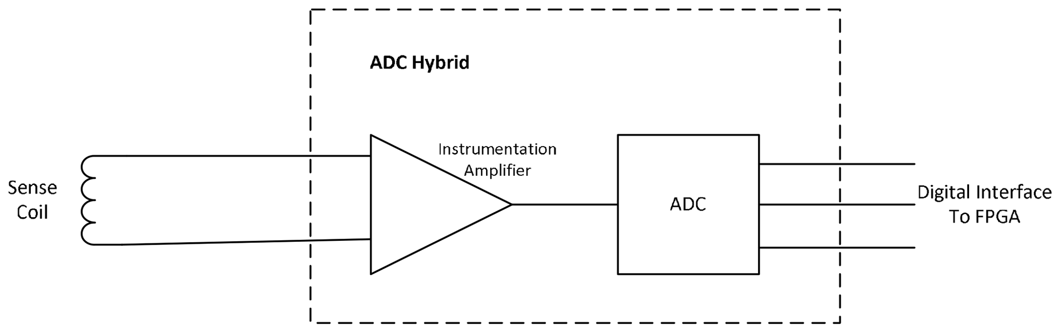
The sensing signal acquisition module circuitry is used to collect the sensing signal. The output signal from the sense coil of the sensor is firstly amplified by the instrumentation amplifier and then sampled and converted by the ADC and transmitted to the FPGA. The block diagram is shown in Fig. 4.

Figure 4 The block diagram of the sensing signal acquisition module.

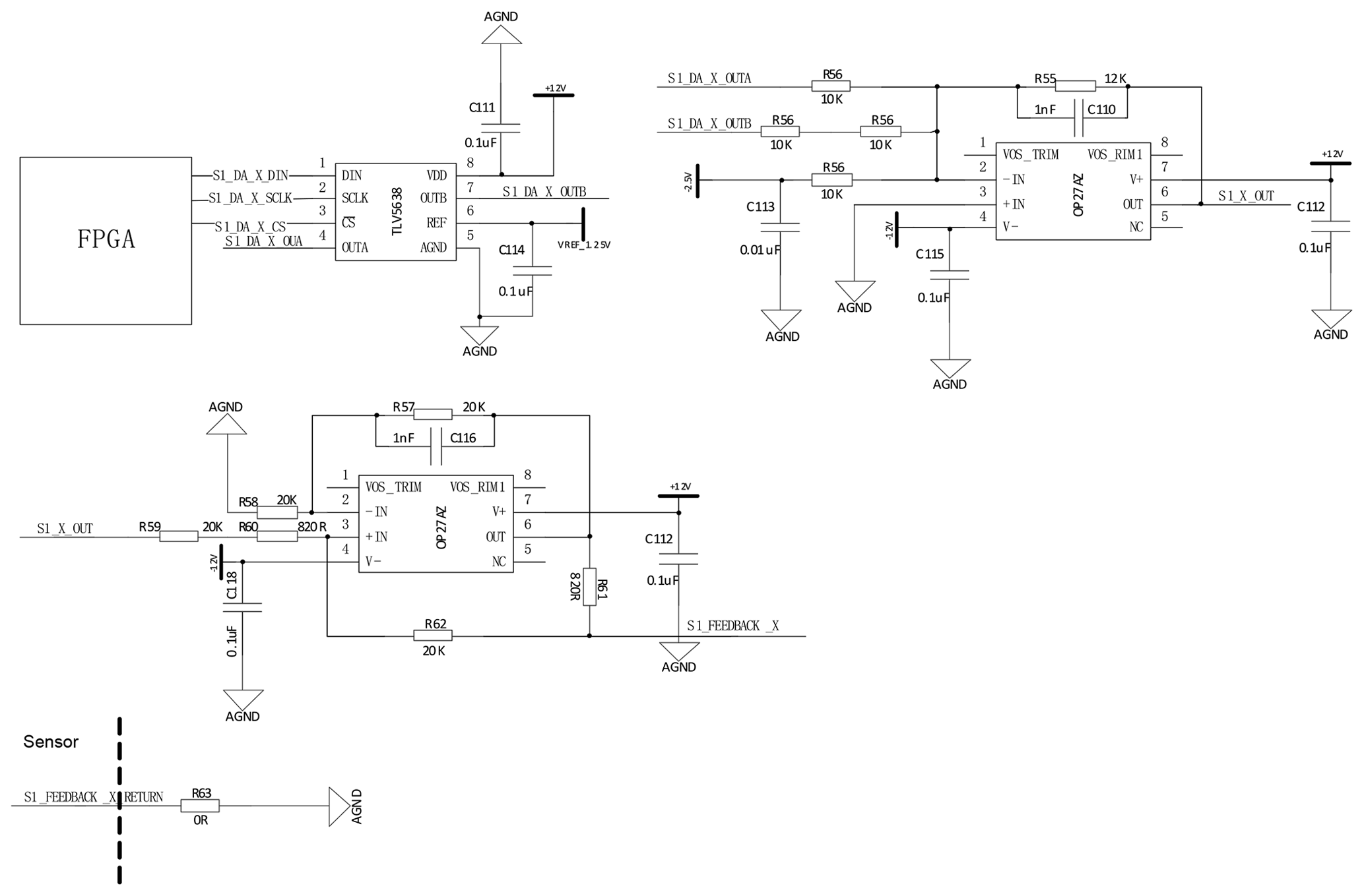
The feedback module circuitry is designed to generate a feedback signal to the feedback coil to form a feedback magnetic field to compensate the external magnetic field. It consists of a DAC circuit and a voltage-controlled constant current source circuit. The 12 bit high-resolution and high-precision DAC contains the anti-interference circuits. The Howland current source circuit built by the operational amplifier is selected to be the voltage-controlled constant current source. A Howland current pump is excellent for putting out a bidirectional current, and it can be used to force currents into sensors in production tests (Pease, 2008). When the resistance is matched, the output resistance tends to be infinite. At this time, the voltage signal is converted into a linear current signal, which is independent of the load and the operating frequency; that is, the output current is a constant and results in a constant compensation magnetic field. We use an “improved Howland” current pump, which can efficiently force as low as microamperes into voltages as large as 10 volts (Pease, 2008). Its block diagram is shown in Fig. 5.

Figure 5 The block diagram of the feedback module circuitry.

The temperature module is designed to collect the voltage divider value of the sensor and the thermistor in the electronics as the temperature value. It is composed of a series voltage divider circuit, ADC chip, and an FPGA. The temperature-measuring circuit consists of a thermistor and a voltage dividing resistor. The ADC chip is responsible for collecting the voltage dividing value of the thermistor, and the FPGA is responsible for controlling the ADC chip for acquisition and encapsulating the collected temperature data into the scientific data packet and then sending it to the payload controller.

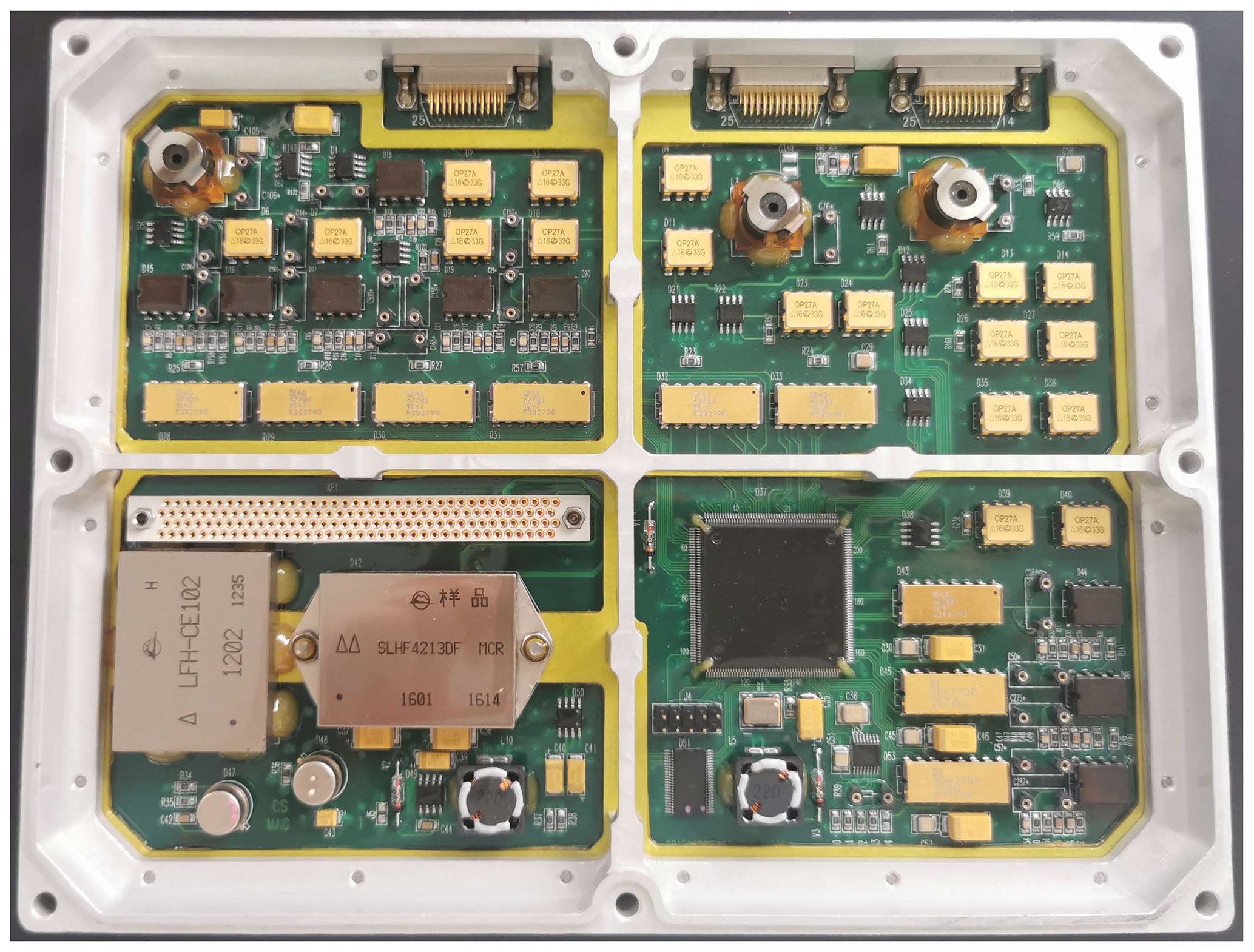
The electronics with the functionalities described above placed on a shared board are shown in Fig. 6. The board area is about 120 cm² and the total power consumption is 0.5 W. The total mass (including the harness) is 1.6 kg.

3 Instrument calibration before launch

3.1 Ground calibration

All the fluxgate magnetometers were well calibrated before launch. The parameters of fluxgate magnetometers to be determined during ground calibration include the scale factor, linearity, frequency response, orthogonality of the triaxial sensor, time stability of the sensor offset, noise of sensor and electronics, and temperature stability of sensor offset. In this section, we will give the detailed calibration processes for determining the calibration parameters mentioned above.

In the absence of an external magnetic field, the strength of the magnetic field given by the magnetometer is considered as the fluxgate magnetometer offset (b), which is systematically independent of sensor and electronics temperature. There is a proportional relationship between the output of each axis of the magnetometer and the real magnetic field. The proportional coefficient is called the scale factor, which is usually different for each axis and independent of the external conditions. The scale factor can be expressed by the following diagonal matrix:

$$\begin{array}{}\text{(1)}& {\mathit{K}}_{\mathrm{SF}}=\left(\begin{array}{ccc}{s}_X& & \\ & s_Y& \\ & & s_Z\end{array}\right).\end{array}$$

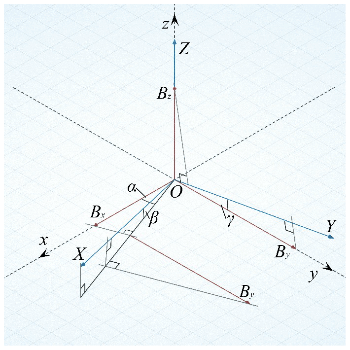
The elements on the diagonal indicate the scale factor of each axis. There is a certain deviation in the direction between the axes of the magnetometer and the ideal Cartesian coordinate system, which leads to the non-orthogonal of in the three sensitive axes of the magnetometer, as shown in Fig. 7, where X, Y, Z is the axes of the magnetometer. We establish an orthogonal coordinate system x-y-z, with the z axis coinciding with the magnetometer´s as the Z axis. The Y axis is in the y–O–z plane. B_x, B_y, and B_z are projections of the magnetic field strength on axes of an orthogonal coordinate system, respectively. The direction error between the magnetometer sensitive axis and the orthogonal coordinate system axis can be represented by three error angles. The angle between the projections of the X axis in the x-O-y plane and the x axis is α, the angle between the X axis and the x–O–y plane is β, and the angle between the Y axis and the y axis is γ. The projection of the magnetic field strength on the three axes of the magnetometer is

$$\begin{array}{}\text{(2)}& \left(\begin{array}{c}{B}_X\\ B_Y\\ B_Z\end{array}\right)={\mathit{K}}_{\mathrm{NO}}\left(\begin{array}{c}{B}_x\\ B_y\\ B_z\end{array}\right),\end{array}$$

where

$$\begin{array}{}\text{(3)}& {\mathit{K}}_{\mathrm{NO}}=\left(\begin{array}{ccc}\cos \mathit{\alpha }\cos \mathit{\beta }& \sin \mathit{\alpha }\cos \mathit{\beta }& \sin \mathit{\beta }\\ & \cos \mathit{\gamma }& \sin \mathit{\gamma }\\ & & \mathrm{1}\end{array}\right).\end{array}$$

The relationship between the magnetometer output B_m and the real magnetic field strength B in the ideal sensor orthogonal coordinate system is

$$\begin{array}{}\text{(4)}& {\mathit{B}}_{\mathrm{m}}={\mathit{K}}_{\mathrm{sf}}{\mathit{K}}_{\mathrm{NO}}\mathit{B}+\mathit{b}.\end{array}$$

Then, B can be expressed as

$$\begin{array}{}\text{(5)}& \mathit{B}=\mathit{K}\left({\mathit{B}}_{\mathrm{m}}-\mathit{b}\right),\end{array}$$

where

$$\begin{array}{}\text{(6)}& \begin{array}{rl}\mathit{K}& ={\left({\mathit{K}}_{\mathrm{sf}}{\mathit{K}}_{\mathrm{NO}}\right)}^{-\mathrm{1}}\\ & =\left(\begin{array}{ccc}{s}_X\cos \mathit{\alpha }\cos \mathit{\beta }& s_X\sin \mathit{\alpha }\cos \mathit{\beta }& s_X\sin \mathit{\beta }\\ & s_Y\cos \mathit{\gamma }& s_Y\sin \mathit{\gamma }\\ & & s_Z\end{array}\right)\end{array}\end{array}$$

if we set

$$\begin{array}{}\text{(7)}& {\mathit{K}}^T\mathit{K}=\left(\begin{array}{ccc}d& e& f\\ e& g& h\\ f& h& i\end{array}\right).\end{array}$$

Figure 6 The fluxgate magnetometer electronics placed on a shared board.

Calculating the modulus of both sides of Eq. (5), we obtain

$$\begin{array}{}\text{(8)}& \begin{array}{rl}\mathrm{d}{B}_{mx}{B}_{mx}& +\mathrm{2}e{B}_{mx}{B}_{my}+\mathrm{2}f{B}_{mx}{B}_{mz}+g{B}_{my}{B}_{my}\\ & +\mathrm{2}h{B}_{my}{B}_{mz}+i{B}_{mz}{B}_{mz}+\\ & \left(-\mathrm{2}\mathrm{d}{b}_x-\mathrm{2}e{b}_y-\mathrm{2}f{b}_z\right)B_{mx}\\ & +\left(-\mathrm{2}e{b}_x-\mathrm{2}g{b}_y-\mathrm{2}h{b}_z\right)B_{my}\\ & +\left(-\mathrm{2}f{b}_x-\mathrm{2}h{b}_y-\mathrm{2}i{b}_z\right)B_{mz}\\ & +\mathrm{d}{b}_x{b}_x+\mathrm{2}e{b}_x{b}_y+\mathrm{2}f{b}_x{b}_z+g{b}_y{b}_y\\ & +\mathrm{2}h{b}_y{b}_z+i{b}_z{b}_z-{\left|\mathit{B}\right|}^{\mathrm{2}}=\mathrm{0}\end{array}\end{array}$$

Equation (8) can be sorted as the following linear equation:

$$\begin{array}{}\text{(9)}& {\left(\begin{array}{c}{B}_{mx}{B}_{mx}\\ \mathrm{2}{B}_{mx}{B}_{my}\\ \mathrm{2}{B}_{mx}{B}_{mz}\\ B_{my}{B}_{my}\\ \mathrm{2}{B}_{my}{B}_{mz}\\ B_{mz}{B}_{mz}\\ -\mathrm{2}{B}_{mx}\\ -\mathrm{2}{B}_{my}\\ -\mathrm{2}{B}_{mz}\\ \mathrm{1}\end{array}\right)}^T\left(\begin{array}{c}d\\ e\\ f\\ g\\ h\\ i\\ {\mathit{K}}^T\mathit{K}\mathit{b}\\ {\mathit{b}}^T{\mathit{K}}^T\mathit{K}\mathit{b}-{\left|\mathit{B}\right|}^{\mathrm{2}}\end{array}\right)=\mathrm{0}.\end{array}$$

If the external magnetic field is kept constant, one can rotate the magnetometer to obtain enough attitudes and Eq. (9) becomes linear equations and K^TK and offset b can be calculated. One can perform the Cholesky decomposition and take the triangular matrix to get K. From Eq. (6):

$$\begin{array}{}\text{(10)}& \left\{\begin{array}{c}{K}_{\mathrm{11}}^{\mathrm{2}}+K_{\mathrm{12}}^{\mathrm{2}}+K_{\mathrm{13}}^{\mathrm{2}}=s_X^{\mathrm{2}}\\ K_{\mathrm{22}}^{\mathrm{2}}+K_{\mathrm{23}}^{\mathrm{2}}=s_Y^{\mathrm{2}}\\ K_{\mathrm{33}}=s_Z\end{array}\right.,\end{array}$$

where s_X>0 and s_Y>0, K_sf can be calculated. From Eq. (6) again we can get

$$\begin{array}{}\text{(11)}& \left\{\begin{array}{c}{s}_Y\sin \mathit{\gamma }=K_{\mathrm{23}}\\ s_X\sin \mathit{\beta }=K_{\mathrm{13}}\\ s_X\sin \mathit{\alpha }\cos \mathit{\beta }=K_{\mathrm{12}}\end{array}\right..\end{array}$$

We can calculate the α, β, γ under the condition that α, β, γ are small angles close to zero.

Table 2 The parameters of the linear calibration for sensors 1–9.

Figure 7 Schematic diagram of non-orthogonal error of the three-axis fluxgate magnetometer.

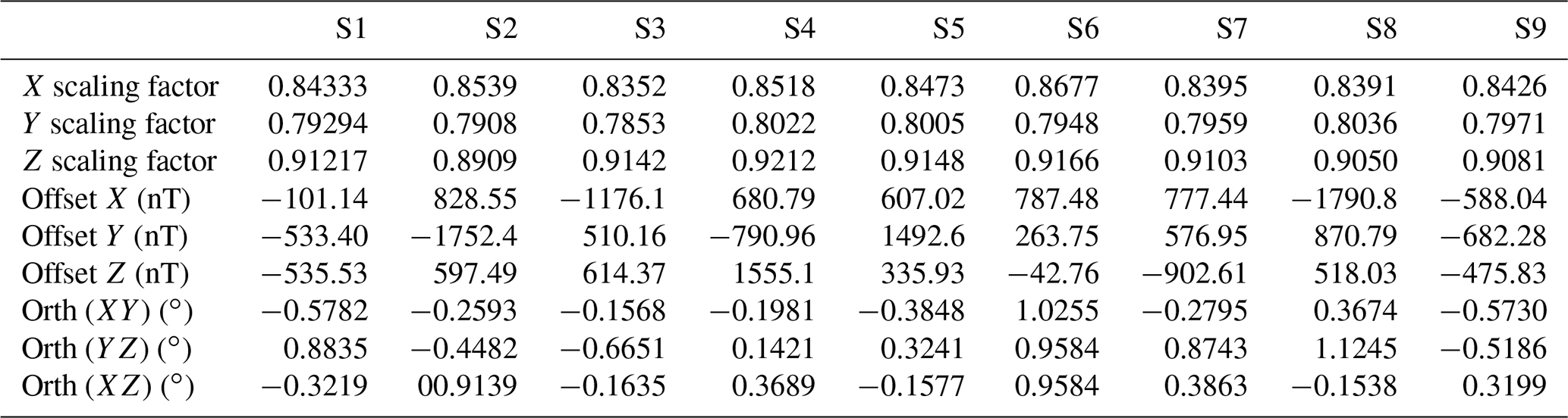
In addition to the above calibration processes, to get sufficient statistics the offset should be measured by sensor rotation in a weak field as often as possible, typically at the beginning and end of each calibration campaign. Table 2 summarizes the calibrated linear parameters of the scaling factor, offset, and orthogonality angle.

The test of the dependency of the magnetometer stability on temperature was performed in a temperature control box in which the temperature varied from −60 to 60^∘. The sensor electronics were mounted inside the temperature control box and the sensor was placed in a Helmholtz coil in which the Earth's magnetic field was decreased by a factor of 10⁴. After the test, the stability of the fluxgate magnetometer is less than 30 pT ^∘C⁻¹ for all sensor axes.

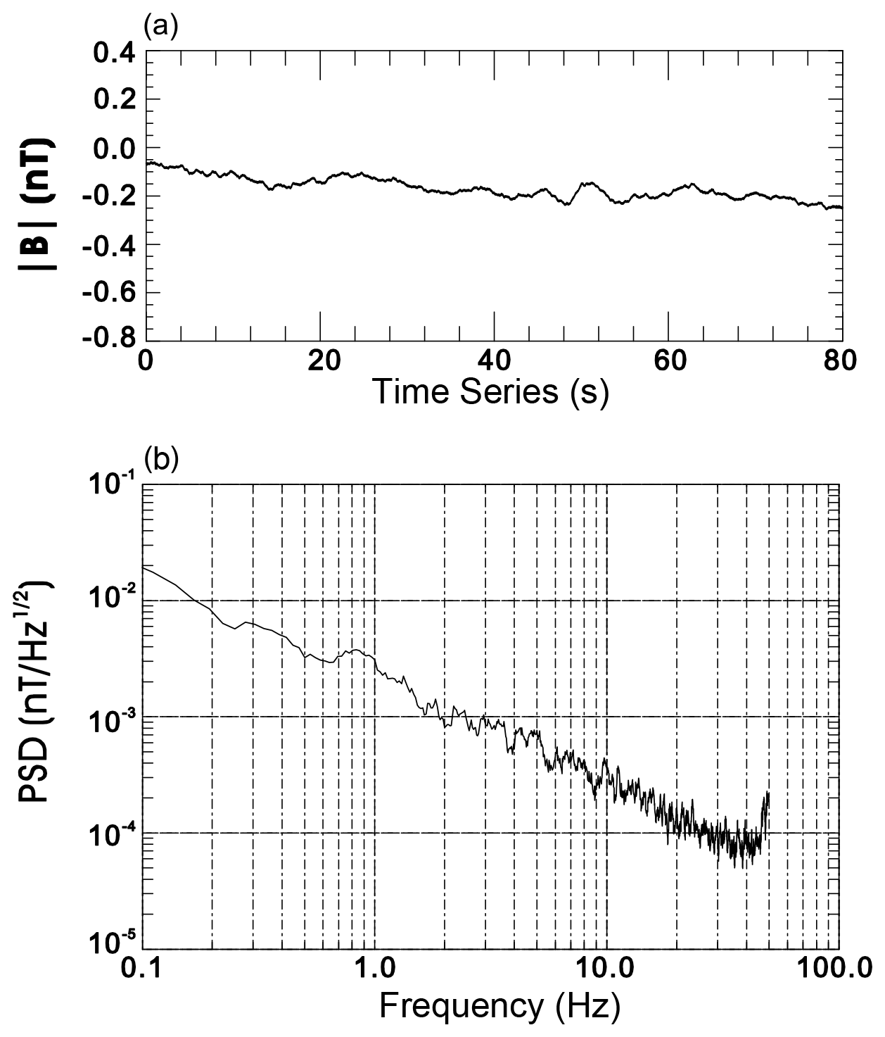
Figure 8 The noise test in a Shielding bucket. (a) The time series of the magnetic field intensity. (b) The corresponding FFT spectrum of the time series.

Figure 9 The noise test in a natural environment. (a) The time series of the magnetic field intensity. (b) The corresponding FFT spectrum of the time series.

The instrument noise was tested in both a Shielding bucket and the natural environment. Figure 8 shows the results of the noise test in a Shielding bucket. Panel (a) shows of time series of 80 s of magnetic intensity measured by the fluxgate magnetometer. The corresponding FFT spectrum is shown in panel (b). As can be seen in panel (b), the noise is about 3 pT $/$ √Hz at 1 Hz. The test results in a natural environment is shown in Fig. 9. The noise is about 10 pT $/$ √Hz at 1 Hz, which is slightly higher than that in a Shielding bucket. The dependency of the sensor and electronics noise on temperature from 0–60 ^∘C were also tested. The noise varies from 20 pT $/$ √Hz at 0 ^∘C to 10 pT $/$ √Hz at 20 ^∘C and to 30 pT $/$ √Hz at 60 ^∘C.

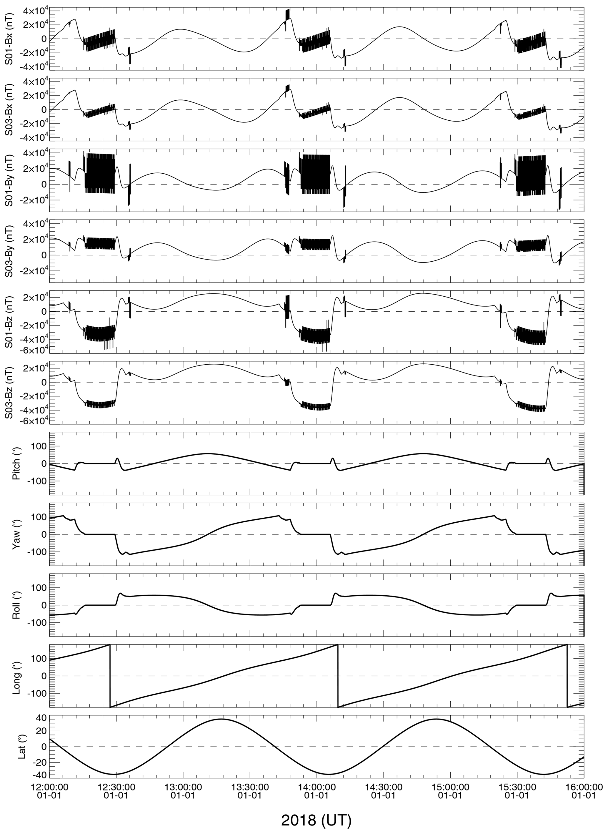
Figure 10 Overview of the raw data of the LOPS-1, including the magnetic data from sensor 1 and sensor 3, the satellite attitude, and orbit.

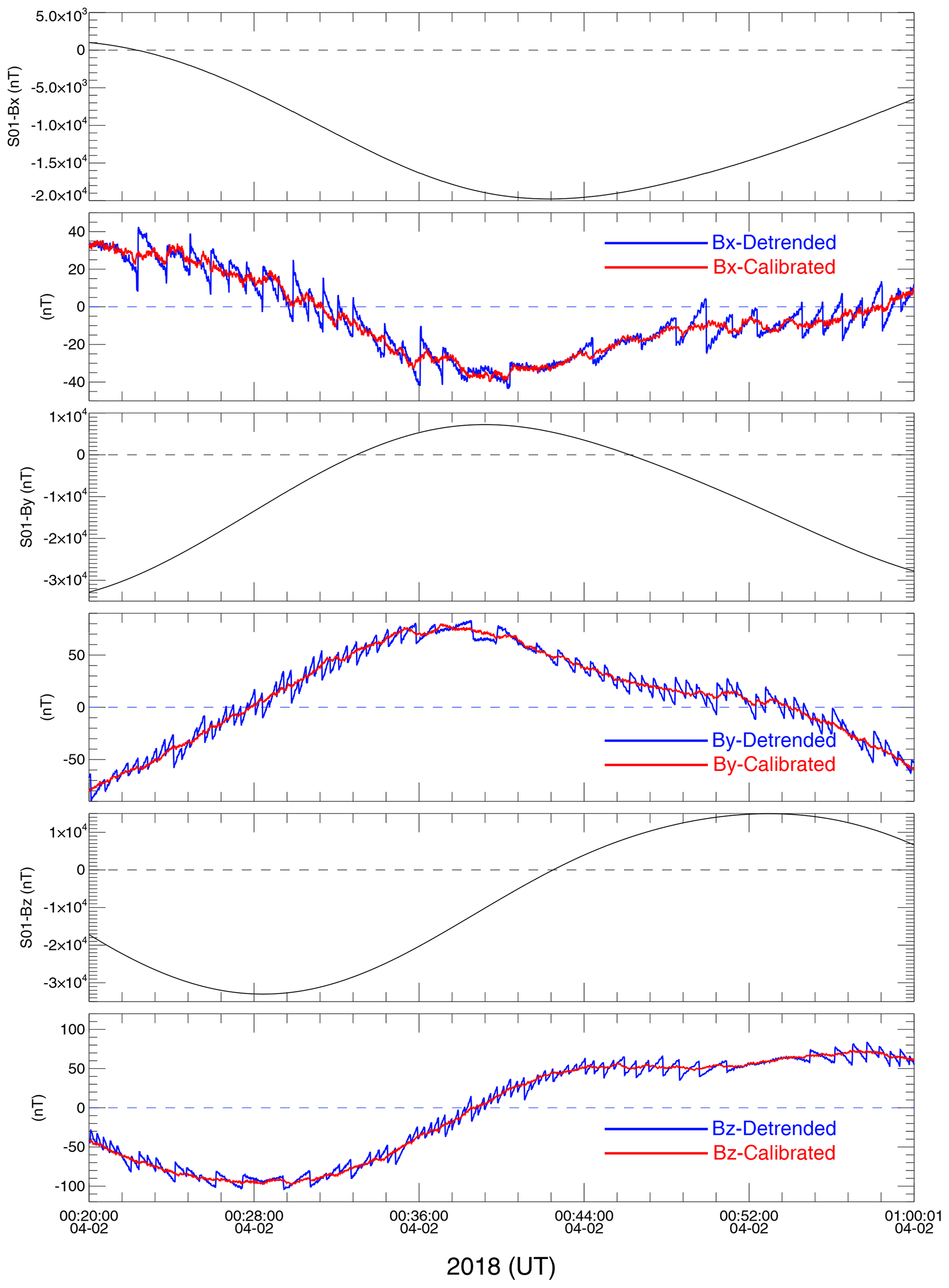
Figure 11 The overview of the LOPS-1 data before (blue) and after dynamic interference correction (red).

3.2 Magnetic survey of the spacecraft

Since the LOPS was not designed to make a strict magnetic cleanliness of the spacecraft, a careful investigation of the spacecraft for both DC and AC fields is needed before launch. Measurements indicate average values of ∼ 900 and ∼ 2000 nT of the AC field at two outboard sensors and the inboard sensor, respectively. There are about 10 nT of dynamic interferences (DC field) at two outboard sensors and ∼ 50 nT at the inboard sensor. These values, though not very accurate, are quite important as the reference for the in-flight calibration of the magnetometers.

4 In-flight calibration: techniques and preliminary results

After the launch of the LOP satellites, we performed the in-flight calibrations, which consist of two categories: one with the spacecraft dynamic interferences (AC field) generated by the electronic current of the spacecraft and the other the static interference (DC field) generated by the hard iron and soft iron material on board the spacecraft. Previous studies have shown that a difference or gradient method based on dual-sensor measurements were proven to be valid in such a calibration (e.g., Zhang et al., 2006, 2007; Auster et al., 2008; Ludlam et al., 2008; Pope et al., 2011). In this section, we will introduce the processes of the calibration techniques of the two interferences and give the preliminary results.

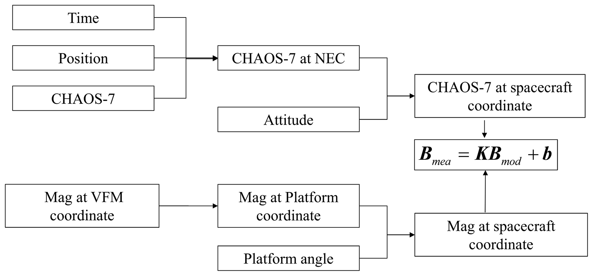
Figure 12 The processes of the static spacecraft interferences estimation based on the CHAOS-7 model.

4.1 In-flight calibration of the spacecraft dynamic interferences

Figure 10 shows an overview of the raw data of the magnetic field observations in the vector field magnetometer (VFM) coordinate along with the attitude and orbit information from the LOPS-1 from 12:00 to 16:00 UT on 1 January 2018. The top six panels show the B_x, B_y, and B_z component from sensors 1 and 3, respectively. The bottom five panels show the three Euler angles (pitch, yaw, and roll), which indicate the satellite attitude and the orbit (longitude and latitude). As we can see in Fig. 9, there are three time intervals in which strong dynamic interferences in magnetic field vector data for both sensor 1 and sensor 3 are observed. The three time intervals coincide with the time periods in which the three Euler angles equal zero. It is noted that the dynamic interferences in sensor 1 are stronger than those in sensor 3. This may be due to the fact that sensor 1 is closer to the satellite antenna, though the two sensors are both 1.5 m away from the satellite platform body. The dynamic interferences are rather small in the other intervals and we exclude the three time intervals in the in-flight calibration processes.

There are several transient signals that are sourced by the spacecraft, such as the antenna effects, the rotation effects of the platform, the solar panel effect, and the electric system of the spacecraft. It should be noted that the spatial gradient of the magnetic field sourced by the spacecraft at the three sensors is obviously larger than the natural magnetic field signal at low-altitude orbit of the Earth. Therefore, the differences of the magnetic field among the three sensors are caused only by the spacecraft dynamic interferences at a fixed time as long as the three sensors were well calibrated before launch and the offsets keep stable at orbit.

$$\begin{array}{}\text{(12)}& {\displaystyle }{B}_{\mathrm{D}\mathrm{12}}\left(t\right)=B_{\mathrm{S}\mathrm{1}}\left(t\right)-B_{\mathrm{S}\mathrm{2}}\left(t\right)\text{(13)}& {\displaystyle }{B}_{\mathrm{D}\mathrm{13}}\left(t\right)=B_{\mathrm{S}\mathrm{1}}\left(t\right)-B_{\mathrm{S}\mathrm{3}}\left(t\right)\text{(14)}& {\displaystyle }{B}_{\mathrm{D}\mathrm{23}}\left(t\right)=B_{\mathrm{S}\mathrm{2}}\left(t\right)-B_{\mathrm{S}\mathrm{3}}\left(t\right)\end{array}$$

In the Eqs. (12)–(14), B_S1, B_S2, and B_S3 are the magnetic fields sourced by the spacecraft at each sensor, respectively. B_D12, B_D13, and B_D23 are the differences of the magnetic field measured by the three sensors and they are only a function of the spacecraft system effect. They contain information about all of the changes in the spacecraft field. Although it is difficult to determine the exact magnetic field sourced by the spacecraft at each sensor, we can identify this signal according to B_D12, B_D13, and B_D23 in the MAG data. In the processes of the dynamic interference correction, the B_D12, B_D13, and B_D23 are the basis of the method to identify the dynamic transient events sourced by the spacecraft. Once the dynamic events are identified, the effect that those dynamic events have on the measured field should be determined and corrected to the data to minimize the effect. After careful examination, we found the magnitude of the differences of the two outboard sensors $\left|B_{\mathrm{D}\mathrm{13}}\right|$ to be substantially smaller than that of the differences between the sensor 2 and sensor $\left|B_{\mathrm{D}\mathrm{23}}\right|$, which is usually an order smaller, indicating that spacecraft dynamic field at the outboard sensor is considerably smaller than that of the inboard sensor. This attenuation is so remarkable that a significant amount of the dynamic interferences sourced by the spacecraft, especially during the intervals in which the spacecraft attitude changes gradually (for example during the interval 12:45–13:45 UT in Fig. 10), are negligible at the two outboard sensors. However, in spite of the reduction, some transient dynamic events should also be calibrated at the two outboard sensors.

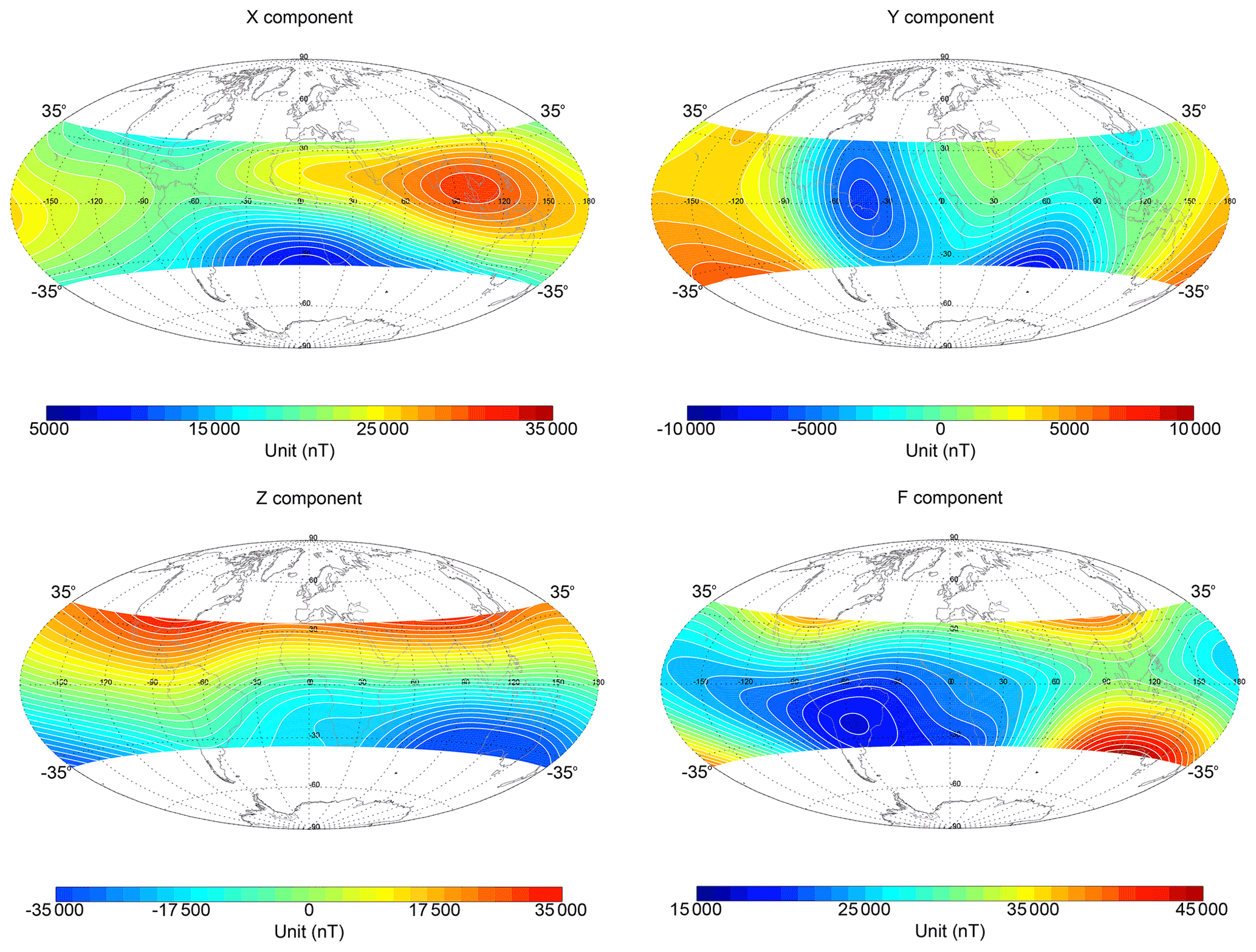
Figure 13 The three magnetic field components and the total intensity at 600 km altitude calculated from the geomagnetic model established based on the LOPS data.

Figure 14 The LOPS magnetic field residuals (after removing the core field given by the CHAOS-7 model) for three components and the field intensity F. The map projection is Hammer–Aitoff.

Figure 11 shows the original magnetic field measurements in the VFM coordinate system, the corresponding detrended fitting (in blue), and the calibrated time series (in red) on board the LOPS-1 in half an orbit during which strong interferences are absent. Due to the strong background magnetic field, the dynamic interferences cannot be well examined in the raw data. Therefore, the detrended time series, which are shown below the corresponding original data, were obtained by subtracting the 120 s smoothed time series. A sawtooth signal can be seen in all three magnetic field components. It is possible that the sawtooth signal is associated with the loading current of the satellite. The current system of the satellite is quite complex so we do not analyze the current itself but diminish its effect mathematically and obtain a reasonable background magnetic field. At first, we obtain the low-frequency components (S_spline) by making a smoothing spline fitting to the original data series. After that, we extract the high-frequency signal (ΔS) by subtracting the low-frequency components from the original data series (S):

$$\begin{array}{}\text{(15)}& \mathrm{\Delta }\mathrm{S}=S-S_{\mathrm{spline}}.\end{array}$$

The sawtooth signals are then contained in ΔS. The first order differences (D_ΔS) of ΔS are calculated and divided into several segments with one segment being about 100 data points. For each data segment of D_ΔS, we determine the threshold above which we treat the data as outliers and set them to be zero. The threshold is set empirically and varies from time to time, but for most of the data we set it to be a value below which there are 85 % of the data points. We then obtain the calibrated high-frequency components by cumulative summation of the new first order difference (D_CAL):

$$\begin{array}{}\text{(16)}& \mathrm{\Delta }{\mathrm{S}}_{\mathrm{CAL}}=\mathrm{CumSum}\left(D_{\mathrm{CAL}}\right).\end{array}$$

Finally, the calibrated data series are the summation of the calibrated-frequency components plus the low-frequency components. This method is just empirical and it will be evaluated as more data are accumulated in the future.

4.2 In-flight calibration of the spacecraft static interferences

Once the dynamic interferences fields were corrected in the spacecraft coordinates, we could estimate the static spacecraft field. Unlike the static spacecraft field of Venus Express, which remains constant throughout the orbit (Pope et al., 2011) and could be estimated using a modified Davis–Smith method (Leinweber et al., 2008), the static spacecraft field of a low-altitude satellite is approximately composed of two parts, with one is a constant generated from the hard iron material and the other an induced magnetic field of the soft iron material and proportional with the background magnetic field. The magnetic fields from a recent CHAOS-7 geomagnetic model (Finlay et al., 2020) were used to estimate the static spacecraft field. The CHAOS-7 model was derived with data only from dark regions, where the interplanetary magnetic field (IMF) B_z averaged over the previous two hours was positive and the IMF B_y was less than +3 nT (Northern Hemisphere) or greater than −3 nT (Southern Hemisphere). The LOPS magnetic field data used to estimate the static field were also selected in the same criteria with the CHAOS-7 model.

Table 3 The parameters to be determined in the calibration model in Eq. (17).

Though the magnetometers on board the LOPS were calibrated on the ground, the parameters (scale factor, linearity, orthogonality of the triaxial sensor, and the offset) of the magnetometers may change to some extent. Therefore, in the estimation of the static field, we also consider those parameters to be determined. The calibration model can be expressed as follows:

$$\begin{array}{}\text{(17)}& B_{\mathrm{mea}}=E_{\mathrm{ma}}{E}_{\mathrm{no}}\left(E_{\mathrm{sf}}\left(B_{\mathrm{earth}}+K_{\mathrm{i}}{B}_{\mathrm{earth}}+B_{\mathrm{p}}\right)+B_{\mathrm{ns}}\right),\end{array}$$

where each variable is listed in Table 3.

Eq. (17) can be rewritten as

$$\begin{array}{}\text{(18)}& B_{\mathrm{mea}}=K{B}_{\mathrm{earth}}+b,\end{array}$$

where

$$\begin{array}{}\text{(19)}& {\displaystyle }K=E_{\mathrm{ma}}{E}_{\mathrm{no}}{E}_{\mathrm{sf}}+E_{\mathrm{ma}}{E}_{\mathrm{no}}{E}_{\mathrm{sf}}{K}_{\mathrm{i}}\text{(20)}& {\displaystyle }b=E_{\mathrm{ma}}{E}_{\mathrm{no}}{E}_{\mathrm{sf}}{B}_{\mathrm{p}}+E_{\mathrm{ma}}{E}_{\mathrm{no}}{B}_{\mathrm{ns}}.\end{array}$$

B_mea and B_earth are the measurements of the magnetometer and the model values of CHAOS-7. Solving the linear Eq. (18), we can obtain K and b:

$$\begin{array}{}\text{(21)}& \begin{array}{rl}& \left(\begin{array}{c}{B}_{\mathrm{mea},x}\\ B_{\mathrm{mea},y}\\ B_{\mathrm{mea},z}\end{array}\right)\\ & =\left(\begin{array}{ccccc}{B}_{\mathrm{mod},x}& B_{\mathrm{mod},y}& B_{\mathrm{mod},z}& \mathrm{0}& \mathrm{0}\\ \mathrm{0}& \mathrm{0}& \mathrm{0}& B_{\mathrm{mod},x}& B_{\mathrm{mod},y}\\ \mathrm{0}& \mathrm{0}& \mathrm{0}& \mathrm{0}& \mathrm{0}\end{array}\right.\\ & \left.\begin{array}{ccccccc}\mathrm{0}& \mathrm{0}& \mathrm{0}& \mathrm{0}& \mathrm{1}& \mathrm{0}& \mathrm{0}\\ B_{\mathrm{mod},z}& \mathrm{0}& \mathrm{0}& \mathrm{0}& \mathrm{0}& \mathrm{1}& \mathrm{0}\\ \mathrm{0}& B_{\mathrm{mod},x}& B_{\mathrm{mod},y}& B_{\mathrm{mod},z}& \mathrm{0}& \mathrm{0}& \mathrm{1}\end{array}\right)\\ & \left(\begin{array}{c}{K}_{\mathrm{1},\mathrm{1}}\\ K_{\mathrm{1},\mathrm{2}}\\ K_{\mathrm{1},\mathrm{3}}\\ K_{\mathrm{2},\mathrm{1}}\\ K_{\mathrm{2},\mathrm{2}}\\ K_{\mathrm{2},\mathrm{3}}\\ K_{\mathrm{3},\mathrm{1}}\\ K_{\mathrm{3},\mathrm{2}}\\ K_{\mathrm{3},\mathrm{3}}\\ b_x\\ b_y\\ b_z\end{array}\right)\end{array}.\end{array}$$

Figure 12 summarizes the estimating processes.

It should be noted that the Euler angles, which describe the transformation from the magnetometer frame to the Star Imager frame, are usually estimated in two ways (e.g., Olsen et al., 2003, 2006):

$$\begin{array}{}\text{(22)}& B_{\mathrm{VFM}}=\mathit{R}\cdot \mathit{T}\cdot B_{\mathrm{NEC}}=-\mathit{R}\cdot \mathit{T}\cdot \mathrm{\nabla }V,\end{array}$$

where B_VFM and B_NEC are the calibrated magnetic measurement in the magnetometer frame and geocentric frame, respectively. R and T are the transformation matrices determined by three Euler angles and attitude transformation matrix given by the Star Imager. In both ways, the estimation of the Euler angle requires both B_VFM and ∇V. However, due to the absence of the absolute magnetic measurements, we could not determine the B_VFM directly; therefore, the Euler angles could not be estimated directly, but are contained in the total compensation parameters K and b (see Eq. 18).

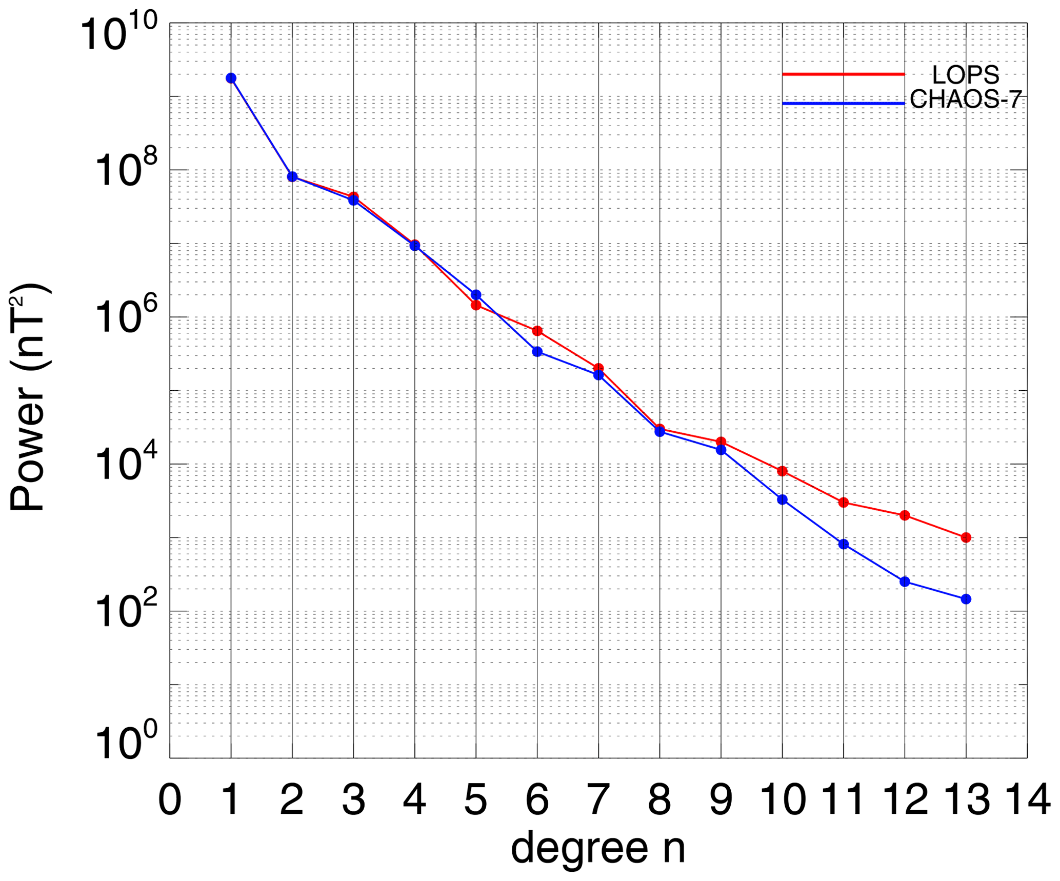
Figure 15 Lowes–Mauersberger spherical harmonic power spectra up to degree n=13 of the vector magnetic field from both the CHAOS-7 model (in blue) and the model based on LOPS data (in red) in April 2018.

Figure 16 The residual north components of different orbits after removing the core field, crustal field, and the magnetospheric field calculated from the CHAOS-7 model. Different colored lines indicate measurements from different orbits. The thick black line referred to the averaged values of all the orbits. Two dashed black lines indicate the standard deviation range.

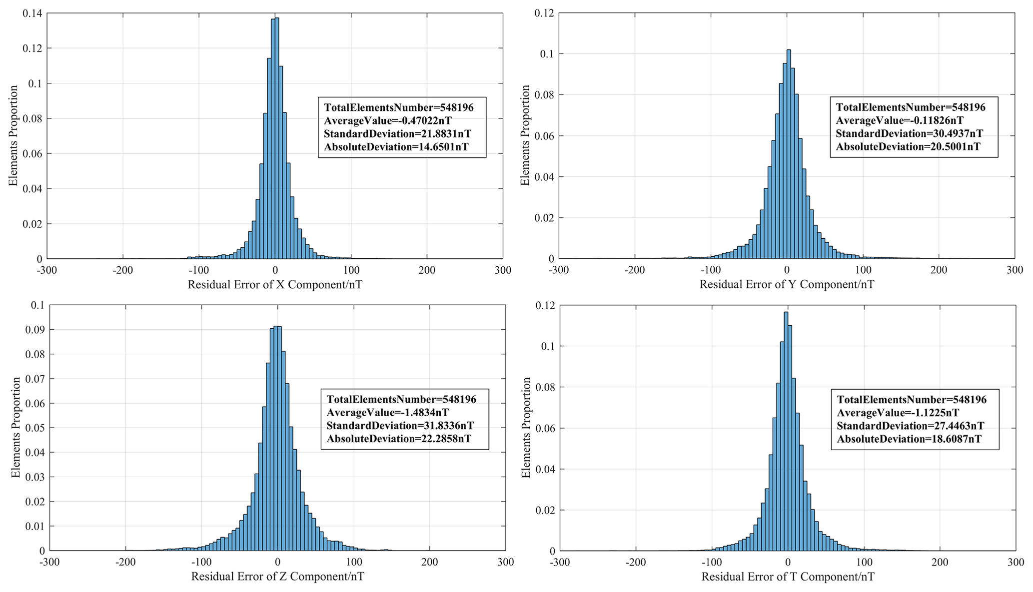
Figure 17 A statistical distribution of the LOPS Magnetic field vector and intensity residual for 1 to 30 April 2018 (after removing the core, crustal, and magnetospheric fields as given by the CHAOS-7 model; Finlay et al., 2020).

4.3 Preliminary results and comparison with geomagnetic models

After the correction of the dynamic and static spacecraft interferences, we can obtain the Earth's natural magnetic vector. Since the observations between the LOPS and SWARM are neither time synchronous nor at the same altitude, we just make a comparison between the observations based on the LOPS geomagnetic model and CHAO-7 model. The data based on the LOPS geomagnetic model was established using the Gaussian spherical analysis based on the vector measurements of 12 satellites during the time period from 1 to 30 April 2018. Data selection criteria for establishing the model is the same as the CHAOS-7 model. In this simple model, we do not consider the geomagnetic secular variation since we only use data in a month. A more comprehensive model with magnetic field data from SWARM, the LOPS, and CSES will be established in the near future in a sequent paper. Figure 13 shows the three magnetic field components and the total intensity (up to spherical harmonic degree n=20) at 600 km altitude calculated from the geomagnetic model established based on the LOPS data. As we can see in this figure, the main features of the geomagnetic main field at 600 km altitude are clearly shown. Figure 14 shows the mean values distribution of the magnetic field residuals (after removing the core, crustal, and large-scale magnetospheric magnetic contributions calculated from the CHAOS-7 model) in the Hammer–Aitoff map projection for the time period from 1 to 30 April 2018. Data with a geomagnetic quiet period (Kp ≤3₀) were selected to make this distribution. As we can see in Fig. 12, despite being quiet periods, the magnetic residuals that describe the external field can be clearly seen in all three components as well as the total intensity. The most remarkable characteristics in the distribution of the X component residual can be seen in Fig. 14a. The X component residual in most of the area covered by the LOPS shows negative values except at the Indian Ocean. There is a clear negative narrow band near the Equator, which may indicate the equatorial electrojet (e.g., Yamazaki and Maute, 2017). A similar feature can also be seen in the F component residual since the equatorial electrojet effect is the most remarkable signature at the low-latitude of 600 km. The Y component residual (Fig. 14b) shows different features, with positive and negative values appearing alternately. This distribution is possible due to the inter-hemisphere field-aligned currents at middle latitudes (e.g., Fukushima, 1994; Lühr et al., 2015). The Z component residual also shows the positive and negative values alternately and it has different features in the Northern and Southern hemispheres. The explanation for this distribution remains unclear.

In order to examine the magnetic power spectra of the vector field calculated from the data based on the LOPS geomagnetic model in Fig. 15, we present the Lowes–Mauersberger spherical harmonic power spectra for both the LOPS-based model and CHAOS-7 model, in which the Gaussian coefficients of the LOPS model were obtained during the period from 1 to 30 April 2018. It is shown that the spectra for the two models decrease steadily from n=1 to 13. From degree n=1 to n=9, the spectra of the two models agree well. After that, the two spectra show differences, with the power spectra of the LOPS model slightly larger than that of CHAOS-7. It is possible that the power spectra of the LOPS with degree n>9 include the magnetic field ingredient of large-scale F-region currents since the spatial scale and the mean amplitude of the magnetic field generated by the currents is overlapped by the core field with degree n=6–13 (see Fig. 3 of Olsen and Stolle, 2012). In addition, we believe that the power spectra also contain the magnetic field ingredient of EEJ, though the spatial scale of the magnetic field generated by EEJ is smaller than the core field with degree n<14. As we know, the EEJ are located at an altitude of about 100–150 km (e.g., Yamazaki and Maute, 2017), which is below the LOPS orbit (600 km). Therefore, in the simple spherical harmonic analysis, the magnetic field generated by the EEJ is treated as the internal field and may not be isolated with the core and crustal field. The strict isolation of the EEJ field will be taken into account by modeling the EEJ and/or data selection in the comprehensive model setup in the future.

We also examined the ability to capture the EEJ by several specific orbits. Due to the limited amount of calibrated data, only a small number of valid events are currently identified. We followed the operation of Alken and Maus (2007) and Lühr et al. (2004) and estimated the core field, crustal field, and field of the magnetosphere by the CHAOS-7 geomagnetic model (Finlay et al., 2020; Olsen et al., 2006). After subtracting the magnetic field of other sources, the measurement was considered to include only the magnetic effects from the ionospheric current system, i.e., the Sq and EEJ effects. The results of the residual north magnetic component for different orbits are shown with different colored lines in Fig. 16. Though a lot of small fluctuations appear in each orbit measurement, a clear EEJ signature with about 20 nT dip at the zero dip latitude could be seen in the thick black line (the averaged value for all the orbits). The asymmetry of the residual magnetic field may be attributed to the spacecraft trajectory, which covers several local times for a specific orbit. Detailed analysis of the EEJ currents captured by our magnetometer measurements will be presented in a subsequent paper.

In order to make a comparison with the CHAOS-7 model, we show the residual distribution of the LOPS magnetic field vector and intensity data during the period from 1 to 30 April 2018 (shown in Fig. 16). The residuals were obtained by removing the core, crustal, and the magnetospheric field as given by CHAOS-7 model. The average values of the residuals are −0.47, −0.12, −1.48, and −1.12 nT for the X, Y, Z components and magnetic intensity, respectively. The absolute deviations are 14.65, 20.50, 22.29, and 18.61 nT for the three components and intensity, respectively. It should be noted that the orbit altitude of the LOPS (∼ 600 km) is slightly higher than that of SWARM B (∼ 530 km). Therefore the CHAOS-7 model values at ∼ 600 km are in fact the magnetic field upward continuation. In addition, it should also be noted that the residuals may contain the magnetic field ingredient generated by the Sq, EEJ, and large-scale F-region currents since those currents are not modeled in the CHAOS-7 model and data on the dayside were not excluded in the residuals calculations.

5 Summary

Benefitting from the good inheritance of the development of the ring cores, the sensor design, and the technology of the electronics, the fluxgate magnetometers on board the LOPS provide the accurate and stable magnetic field measurements of the Earth at low-orbit after removing both the dynamic and static interferences sourced by the spacecraft. The Large amount of measurements from 45 magnetometers on board 15 satellites lead to a major challenge of data calibration as well as scientific analysis. On the other hand, with unprecedented spatial coverage of the magnetic field measurements and the data accumulation, it also presents opportunities to study the magnetic field of the Earth in great detail, especially the electric current system at mid- to low latitude, such as the ring current and the EEJ, which is quite important for separation of the internal and external magnetic field for establishing more accurate geomagnetic models.