the Creative Commons Attribution 4.0 License.
the Creative Commons Attribution 4.0 License.
 | 03 Nov 2021
Evaluation of multivariate time series clustering for imputation of air pollution data
Iain Lake
Claire E. Reeves
Beatriz De La Iglesia
Air pollution is one of the world's leading risk factors for death, with 6.5 million deaths per year worldwide attributed to air-pollution-related diseases. Understanding the behaviour of certain pollutants through air quality assessment can produce improvements in air quality management that will translate to health and economic benefits. However, problems with missing data and uncertainty hinder that assessment.
We are motivated by the need to enhance the air pollution data available. We focus on the problem of missing air pollutant concentration data either because a limited set of pollutants is measured at a monitoring site or because an instrument is not operating, so a particular pollutant is not measured for a period of time.
In our previous work, we have proposed models which can impute a whole missing time series to enhance air quality monitoring. Some of these models are based on a multivariate time series (MVTS) clustering method. Here, we apply our method to real data and show how different graphical and statistical model evaluation functions enable us to select the imputation model that produces the most plausible imputations. We then compare the Daily Air Quality Index (DAQI) values obtained after imputation with observed values incorporating missing data. Our results show that using an ensemble model that aggregates the spatial similarity obtained by the geographical correlation between monitoring stations and the fused temporal similarity between pollutant concentrations produces very good imputation results. Furthermore, the analysis enhances understanding of the different pollutant behaviours and of the characteristics of different stations according to their environmental type.
- Article
(4956 KB) - Full-text XML
- BibTeX
- EndNote


Time series (TS) analysis has received much attention in recent decades due to its importance in many real-world applications such as earthquake prediction (Di Bello et al., 1996), weather forecasting (Carbajal-Hernández et al., 2012), air pollution forecasting (Du et al., 2020), and human activity recognition (Seto et al., 2015). Generally speaking, TS data can be described as a sequence of observations that a variable takes over time. When several variables are observed and recorded simultaneously, this becomes a multivariate time series (MVTS).
The quality of the air in the UK is assessed based on five main pollutants. In this study we focus on the four main pollutants: particulate matter less than 2.5 µm in diameter (PM2.5) or less than 10 µm in diameter (PM10), ozone (O3), and nitrogen dioxide (NO2). These pollutants are measured hourly at various monitoring stations.
The main challenge with analysing these pollutant TS is that not all the stations report all the pollutants. Even if a station does, it may not measure a particular pollutant all the time due to instrument downtime. In our previous work (Alahamade et al., 2021), we applied an intermediate fusion approach to fuse the distance between stations using the similarity of the four pollutants. The similarity between pollutant TS was measured using shape-based distance (SBD) between hourly pollutant concentrations (TS), as we found that SBD is better than other measures on our dataset (Alahamade et al., 2020). Then we used the k-means clustering algorithm to cluster the stations based on the fused distance; we called that MVTS clustering. Our initial clustering analysis showed that using the basic k-means with the fused distance gives very compact geographical clustering that enhances our understanding of the UK's air pollutant behaviours. Adding to that, using the fused distance to measure the similarity between the pollutants helped us solve some of the uncertainty problems associated with missing pollutant values as the MVTS clustering enables imputation even when no measurement is available for a given pollutant. This is because the multivariate nature of the clustering enabled a station to be allocated to a cluster based on the value of the other pollutants measured.
Based on the clustering results and station geographical location, we proposed three models to impute the whole time series for the missing pollutant at a given station. In this paper, we apply multiple model evaluation functions to assess which model gives the best results and to demonstrate the validity of our models.
Our long-term goal is to reduce the uncertainty in air quality assessment by imputing all missing pollutants in the monitoring stations. This will allow us to calculate new air quality indices that may or may not agree with the previous indices; that is, the observed indices that incorporate missing data. This in turn will help us to identify where more measurements can be beneficial.
We refer to our approach as time series imputation because we used the observed time series to impute missing time series (whole TS) in stations where one pollutant is not measured but other pollutants are. In this process, we are not filling the missing values within the time series (e.g. interpolating) but imputing a new TS. Also, we do not use predictive models; hence, we do not consider this a prediction task. However, it could be argued that our task is close to spatial interpolation (Lam, 1983) even though it is not completely based on spatial information; that is, we did not use any geographical information within the proposed MVTS clustering. Geographical information, however, is used in nearest-neighbour approaches, which are used in the ensemble proposed. Nevertheless, the main goal of the spatial interpolation is to fill in the gaps (points and/or locations with unknown measurements) using points with known values to cover a certain geographical area (Lam, 1983). Our goal is to impute unmeasured pollutants (whole TS) in several stations where they are not measured using the fused similarity between stations of other pollutants or using an ensemble of techniques including the MVTS clustering approach. We would argue that our imputation approach incorporates some uncertainty by using a combination of values (within the clustering process and within the ensemble) to produce the imputed value.
The paper's structure is as follows: Sect. 2 discusses some of the existing TS clustering methods and their application in the air quality field. Section 3 gives a brief introduction of the air quality assessment in the UK and its challenges. Section 4 discusses all the methods we used in detail to impute the missing pollutants and evaluate our proposed solutions. Finally, in Sect. 5, we analyse the results of our imputation models. Then, we conclude the work with some final remarks and indication for further developments in Sect. 6.
In this section, we briefly review some representative research in clustering techniques and its application in air pollution modelling. Data mining techniques have been widely applied to study air pollution data; however, most of this research focuses only on a single pollutant (univariate TS), while clustering multivariate time series remains a challenging task (Liao, 2005). Partitioning algorithms such as k-means and k-medoids are very common among works related to TS clustering and have been applied in many papers (e.g. Ignaccolo et al., 2008; Austin et al., 2013; Tuysuzoglu et al., 2019)
Austin et al. (2013) used the k-means algorithm to identify spatial patterns in air pollution data to cluster US cities based on the similarity of their PM2.5 composition profiles, then characterize these clusters based on chemical characteristics, emission profiles, geographic locations, and population density. Ignaccolo et al. (2008) transformed the TS of pollutant daily observations into a functional form to smooth the TS, then classified the air quality monitoring network in northern Italy using the partitioning around medoids algorithm (PAM) to cluster three individual pollutants, namely NO2, PM10, and O3. Tuysuzoglu et al. (2019) applied different clustering algorithms such as k-means, expectation maximization, and canopy for each air pollutant in the dataset (NO, NO2, SO2, PM10, and O3), then aggregated the clustering results based on majority voting to identify one clustering solution for similar regions in terms of air quality.
On the other hand, there has been some research into similarity within MVTS. For example, Fontes and Budman (2017) proposed an MVTS clustering method based on extracted features from the univariate TS. In their work, principal component analysis (PCA) is used to measure the similarity between MVTS, and fuzzy k-means is used to cluster these TS. This clustering approach was used for fault detection in a gas turbine. Zhou and Chan (2014) developed an algorithm for clustering MVTS by discovering each TS's temporal patterns. Their algorithm is based on k-means and aims to groups MVTS with similar temporal patterns together into the same cluster. D'Urso et al. (2018) proposed robust fuzzy clustering models for MVTS based on an exponential transformation of the dissimilarities. This algorithm was applied to real-world data on the concentrations of three pollutants (NO, NO2, and PM10) in the Metropolitan City of Rome for the problem of detecting pollution alarms.
In our previous work (Alahamade et al., 2020), we compared different TS distance measures and imputation techniques to impute missing observations and missing pollutants (TS). We found that using shape-based distance (SBD) gives better separated clusters than dynamic time warping (DTW). Also, using MICE to impute the TS missing observations is better than using some single imputation methods such as simple moving average (SMA). We used a univariate TS clustering using k-medoids (PAM) to cluster stations and imputed the missing pollutants using the cluster average. In this work, we use the k-means clustering algorithm and include a number of pollutants in the clustering, which makes it MVTS clustering. This clustering algorithm was proposed in Alahamade et al. (2021) where more details can be found. Here we extend that work by applying the imputation solution to real data and using extensive evaluation methods to demonstrate its effectiveness. This enables us to extend our understanding of pollutant behaviour.
We will study air pollution using the concentrations measured at the Automatic Urban and Rural Network (AURN) around the UK. The stations in the network are automatic and produce hourly pollutant concentrations. The data are collected and stored, then made directly available via the Web (DEFRA, 2021). There are 167 stations with different environmental types: rural, urban, suburban background, roadside, and industrial.
The Daily Air Quality Index (DAQI) represents air pollution levels in the UK. This index is reported based on the highest individual DAQI derived for each of the five major air pollutants (O3, NO2, PM10, PM2.5, and SO2) based on their concentrations. If concentration data for some of these pollutants are not available, the DAQI is based on those pollutants for which data are available. The DAQI is used to provide an indication of the air quality and some associated information that may be used by at-risk groups as well as the general population (DEFRA, 2021). The DAQI is numbered from 1 to 10 and divided into four bands: “low” (1–3), “moderate” (4–6), “high” (7–9), and “very high” (10). The air quality is negatively correlated with the DAQI, meaning that a higher DAQI represents worse air quality.
The MVTS clustering algorithm and our proposed imputation models were implemented in R version (3.5.2) and are fully explained in previous work (Alahamade et al., 2021). To provide a more robust testing scenario, we separate the “model building” stage from the imputation testing stage. We use an initial data period of 3 years (2015–2017) as a training set to build the clustering and then impute on the next year (2018) of the TS to evaluate the goodness of fit.
4.1 Imputation models of missing pollutant TS
For evaluation purposes, we assume each pollutant from each station is missing entirely and impute it. For any given station, j, to impute the values of missing pollutant , where i represents the different pollutants (), we use different models under two main similarity criteria: the similarity using clustering solutions and the similarity using geographical distance.
The k-means clustering algorithm is used to group the stations based on their temporal similarity, which is the similarity in time between the hourly pollutant concentrations using SBD as the temporal distance measure. This distance function is implemented in the “dtwclust” package in R (Sarda-Espinosa, 2017). The geographical distance is used to find the spatial similarity between station locations. Adding to that, we use an ensemble model which calculates the median of all the previous imputation models; this model aggregates the temporal and spatial imputation using both the time series clustering and the geographical location similarity. Then, we evaluate these models to select the one that gives the highest similarity to the real values which are known. We explain these models in detail in the following sections.
4.1.1 Imputation models using clustering results
Once a clustering of our stations is obtained, we can use the clustering solution to impute missing TS (pollutants). If station j belongs to cluster Cx, (, where k is the number of clusters) given the measured pollutants over time, then, to impute pollutant Pi based on the clustering results, we use three models.
-
We impute the average of pollutant Pi in cluster Cx, which is the hourly average of pollutant Pi in all the stations that fall in this cluster. We call this method cluster average (CA).
-
We impute the average of pollutant Pi in cluster Cx, but using only stations with the same environment type to station j within the cluster, such as “background rural”, “background urban”, “traffic”, or “industrial”. We call this method CA+ENV. This is in recognition of the fact that the type of station may be important and result in more similar pollutant concentrations.
-
We impute the average of pollutant Pi in cluster Cx for stations that belong to the same region. As defined by DEFRA (DEFRA, 2021) there are 16 regions in the UK for air quality assessment, such as eastern and northern Wales, the East Midlands, and the other UK regions; this method is called CA+REG.
4.1.2 Imputation models by similarity using geographical distance
First, we measure the geographic distance using the Harvison metric, which calculates geographic distance on Earth based on longitude and latitude. We calculate the distance between station j and all other stations that measure pollutant Pi. Then to impute pollutant Pi for station j we use the following:
-
the nearest neighbour (1NN) using the Harvison-based distance to station j – this method is called 1NN; and
-
the average of the two nearest neighbours (2NN) to station j – this method is called 2NN.
4.1.3 Imputation model by ensemble
In this approach, for a given station j, to impute pollutant Pi, we use the median value of all the imputed values from the previous models. Those are cluster average (CA), cluster average considering the station type (CA+ENV), cluster average considering the region (CA+REG), first nearest neighbour (1NN), and the average of the two nearest neighbours (2NN). This method is called Median. This imputation approach may be computationally the most expensive as it needs for all others to be computed, but ensembles have the potential to provide very powerful solutions by combining predictions.
4.2 Imputation model evaluation
We evaluate how plausible the imputation is using different models by comparing truth values to imputed values. The model evaluations are based on the test dataset, which is the 2018 data. As mentioned earlier we do this by taking each existing TS for which we have values, one at a time, and consider them missing. We impute the whole TS by various models and compare that to the ground truth. We are evaluating our models against the real concentrations which contain missing values; hence, we ignore all the missing values in this evaluation. For each model, we can average the different imputation models' behaviour from all the stations to establish the one that provides imputed values closest to the real values. Hence, for our experimental set-up we take each existing TS for a given pollutant and station, , in turn and impute it by the various models to obtain an imputed TS, . We compare the real values to the imputed values using different statistical and graphical model evaluation functions. The statistical functions include the fraction of predictions within a factor of 2 (FAC2), mean bias (MB), normalized mean bias (NMB), root mean squared error (RMSE), coefficient of correlation (R), and index of agreement (IOA). These measures are used to evaluate the temporal variation of air pollutants between imputed–modelled and observed concentrations. The graphical functions include a conditional quantile plot, time variation plot, and Taylor diagram. These are functions within the “openair” package, a freely available air quality data analysis tool in R (Carslaw and Ropkins, 2012) that presents comparisons between the modelled and measured air pollutant concentrations and their statistics graphically. We use the R packages openair (Carslaw and Ropkins, 2012) and tidyverse (Wickham et al., 2017) for the evaluation.
Model evaluation functions are beneficial when more than one model is involved in the comparison and help us in understanding why a model does not perform well. The model that gives the lowest error on average, the highest correlation, and the highest degree of agreement between imputed and observed concentrations for all stations (i.e. imputed TS) is initially considered the best model. However, extensive evaluation with various graphical functions enables us to better assess the model quality and how it reflects uncertainty. Note that the best model may change from one pollutant to another and may be affected by other factors such as station type (e.g. urban background, rural, and roadside) or pollutant lifetime and spread.
4.3 DAQI calculation
In the UK, DAQI forecasts are issued on a national scale; they are produced by the Met Office in the morning for the current day as well as for the next 4 d. The forecast is improved by incorporating the recent observations of air quality recorded at the AURN stations. The overall air pollution index for a site or region is determined by the highest DAQI of the five pollutants. The regional DAQI is the highest index among all the stations in that region.
For our evaluation, we calculated the daily DAQI value using the observed data for each station. This is because the DAQI value is not saved as part of the historical data available, so we need to calculate it from the downloaded data. DEFRA has published a guide for the implementation of DAQI (DEFRA, 2013), which explains how the value is calculated, and we follow that guidance. To calculate DAQI, each air pollutant is calculated as follows.
-
Ozone. The O3 is measured hourly. To determine the DAQI we need to calculate the daily maximum 8-hourly running mean concentration. First, for each hour we calculate the running 8-hourly mean from the previous hours. Then we find the maximum value of these 8-hourly running means. For this calculation 75 % of the data must be captured to calculate the 8-hourly mean.
-
Nitrogen dioxide. The NO2 is measured based on an hourly mean. We calculate the daily NO2 contribution to the DAQI by taking the maximum observation in 24 h every day from 00:00 to 23:00 GMT.
-
Particle PM10 and PM2.5. These are measured hourly. The DAQI is based on the 24 h mean, which we calculate by taking the mean value from the hourly observations. For these pollutants 75 % of the daily observations must be captured to calculate the mean; otherwise, the pollutant is considered missing that day.
-
We define the daily index for each pollutant separately. Then, for a station, we take the highest air pollutant index to be the value of the DAQI at that station.
We called the DAQI that is calculated based on observation “observed DAQI” and the DAQI that is calculated based on imputation “imputed DAQI”. We use the observed DAQI as a performance tool to evaluate our imputation model on its ability to reproduce the Daily Air Quality Index. Note that although we produce only one imputation and not multiple imputations at this stage, we believe they reflect the underlying uncertainty because they are based on a number of aggregated methods.
In this section, we first analyse the proposed pollutant imputation models using some statistical and graphical air pollution modelling evaluation functions. Then, we evaluate the imputation model performance based on the comparison between the observed and imputed DAQI.
5.1 Air pollution imputation modelling evaluation
We first evaluate imputation models based on the statistical and then on the graphical analysis.
5.1.1 Model evaluation based on statistical analysis
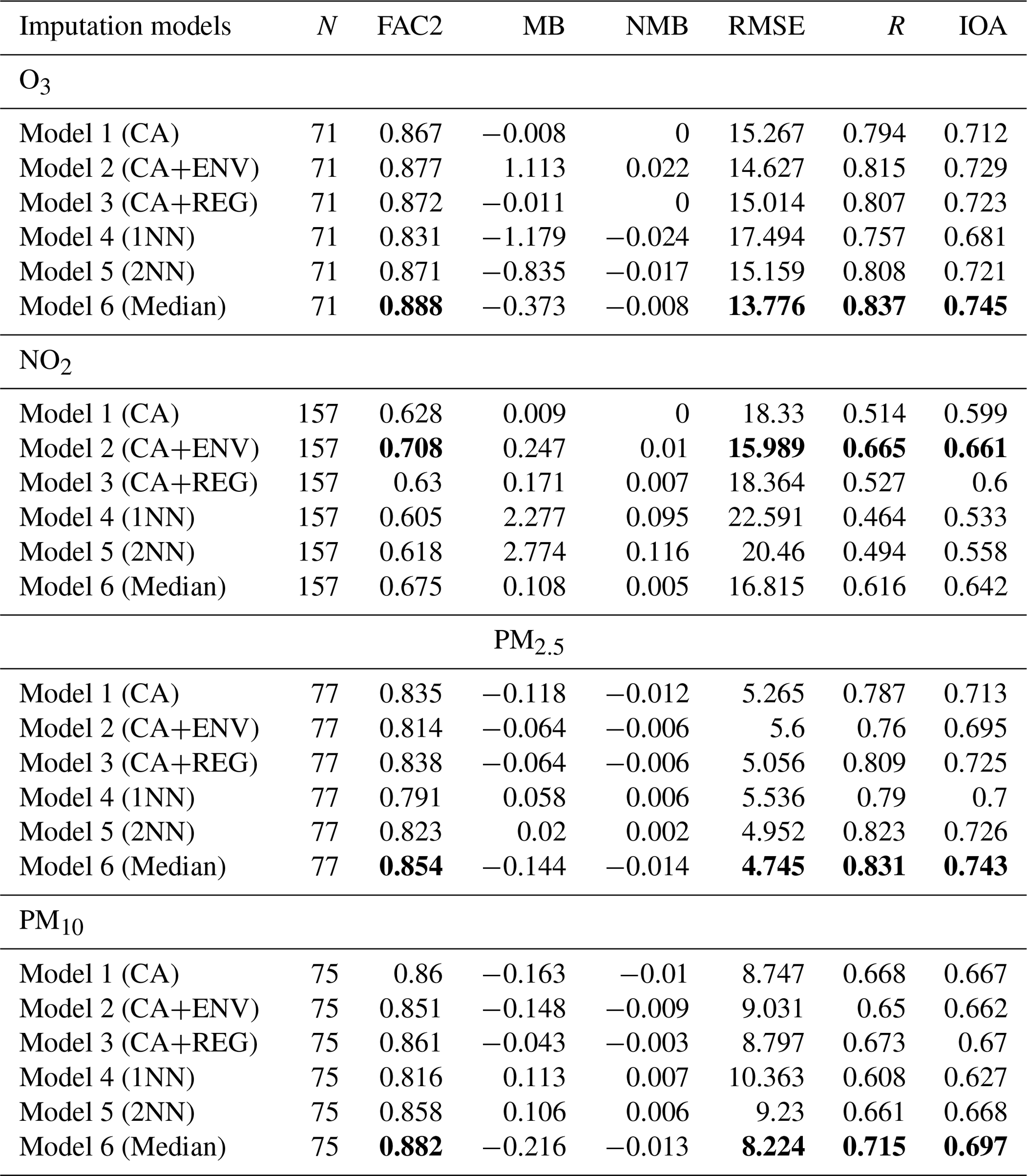
Table 1 shows the statistical analysis results. In this table N is the number of stations that measure each pollutant. The table also shows the fraction of predictions within a factor of 2 (FAC2), mean bias (MB), normalized mean bias (NMB), root mean squared error (RMSE), coefficient of correlation (R), and index of agreement (IOA).
In general, model 6 (Median), which is the model that uses the ensemble technique of other models, gives the lowest error average (RMSE), the highest Pearson correlation coefficient (R), and the highest agreement between imputed and observed concentrations (IOA) for O3, PM2.5, and PM10. However, NO2 shows different behaviour, with model 2 (CA+ENV) achieving slightly higher performance with an increase in the correlation coefficient (by 0.049) and decrease in error average (by 0.826) compared to model 6 (Median). The model bias (MB) for model 2 is 50 % higher than that of model 6. NO2 shows local patterns, as it is concentrated where it is emitted in urban areas and near the roadside. Adding to that, NO2 is shorter-lived than other pollutants and shows greater spatial variability, with concentrations being strongly influenced by the environment type (e.g. roadside, urban background, rural). This changes the NO2 concentrations from one location to another based on the environmental type (CenterForCities, 2020).
All the selected models performed well, with 71 %–89 % of their imputations falling within a factor of 2 of the observed concentrations as shown in the FAC2 values in Table 1. According to Derwent et al. (2010), an air quality model minimum requirement is that the FAC2 value is higher than 0.50 and NMB values should be in the range between −0.2 and +0.2. Both are met by our models. NMB measures if the model underpredicts or overpredicts, as it estimates the difference between the mean observed and imputed concentrations. Negative NMB means that the model underpredicts and vice versa. All the models have very small biases.
Table 1Performance of the hourly pollutant concentration imputation models based on statistical measures. Best values are in bold for FAC2, RMSE, R, and IOA.
5.1.2 Model evaluation based on Taylor diagram analysis
We use a Taylor diagram to analyse three main statistics: correlation coefficient R, the standard deviation (sigma), and the root mean square error (centred). These statistics can be plotted on one (2D) graph, which can be represented through the law of cosines (Taylor, 2001).
The standard deviation represents the variability between modelled and observed concentrations. The observed variability is plotted on the x axis. The magnitude of the variability is measured as the radial distance from the plot's origin. The black dashed line shows this for the observed value. The grey lines are isopleths for the correlation coefficient (R) as indicated by the arc-shaped axis; the correlation increases along the arc towards the x axis. The centred root mean square error (RMSE) is represented by the concentric brown dashed lines. The further the points or models are from the observed value, the worse performance they have (Carslaw and Ropkins, 2012). Figure 1 shows Taylor diagram plots for all models with all pollutants.
In almost all cases the models exhibit less variability than observed, as indicated by the points being closer to the origin than the black dashed line. In general, model 4 (1NN) followed by model 5 (2NN) show variability that is most similar to the observations, as indicated by their relative closeness to the black dashed line. However, these models tend to have the lowest correlation coefficients, as indicated by the grey lines, and the greatest RMSE, as indicated by the brown dashed lines. Models 4 and 5 use the concentrations from a single site (i.e. the nearest stations) in the imputation, whereas the other models use a cluster average (CA, CA+REG, CA+ENV) or a model ensemble average (Median), so it is reasonable for models 4 and 5 to have variability fairly similar to the observed concentrations. All the other models display less variability than the observed concentrations (as indicated by their points being further from the black dashed line); this may be consistent with their derivation methods, which may smooth out some of the variability.
Model 6 (Median), regardless of its ability to capture variability, is confirmed as having the highest correlation coefficient and the lowest centred root means squared with all the pollutants except NO2, for which it is the second-best behind model 2 (CA+ENV).

Figure 1Taylor diagrams comparing modelled and observed concentrations for O3, NO2, PM2.5, and PM10.
5.1.3 Model evaluation based on conditional quantile analysis
We analyse the spread of the modelled and observed pollutant concentrations using conditional quantile plots. Figures 2 and 3 show the conditional quantile plots for the six imputation models (panels a to f). This visualization splits the concentrations into bins according to values of the modelled concentrations. The median line of these values as well as the 25th 75th and the 10th 90th quantile values are plotted together with a blue line showing a “perfect” model. Also shown are histograms of modelled concentrations (shaded grey bars) and histograms of observed concentrations (blue outline bars).
These plots show how the modelled concentrations compare with the observed concentrations and how the models capture the variability in the concentrations. The spread of the modelled concentrations around the perfect model line (blue line) is shown by the shaded portions and quantile intervals. If narrow, it indicates high agreement or precision between the modelled and observed concentrations. The quantile intervals also represent the uncertainty bands. In some cases these intervals do not extend along with the median line due to insufficient concentrations to calculate them. The model with good performance is obtained when the median (red line) coincides with the perfect model (blue line) and when the spread in the percentile is as narrow as possible.
From these plots, in general, the histograms indicate that model 4 (1NN) (panel d) has better estimation of the variability between the observed and modelled concentrations, as observed before, even though the median line does not match the perfect model. This model is positively biased at high concentrations, as shown by the departure of the median line below the blue line for all pollutants. This result supports our analysis from the Taylor diagram that model 4 (1NN) has the lowest variability between modelled and observed concentrations, but with a lower correlation coefficient, and the highest centred root means squared for all pollutants.
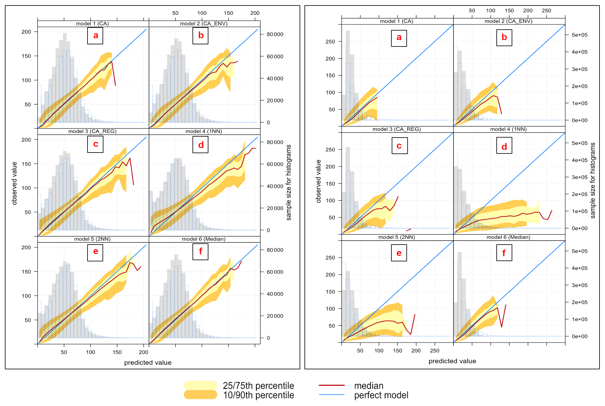
Figure 2Conditional quantile plot of modelled and observed pollutant concentrations of O3 (left plot) and NO2 (right plot) for proposed imputation models: (a) model 1 (CA), (b) model 2 (CA+ENV), (c) model 3 (CA+REG), (d) model 4 (1NN), (e) model 5 (2NN), (f) model 6 (Median).
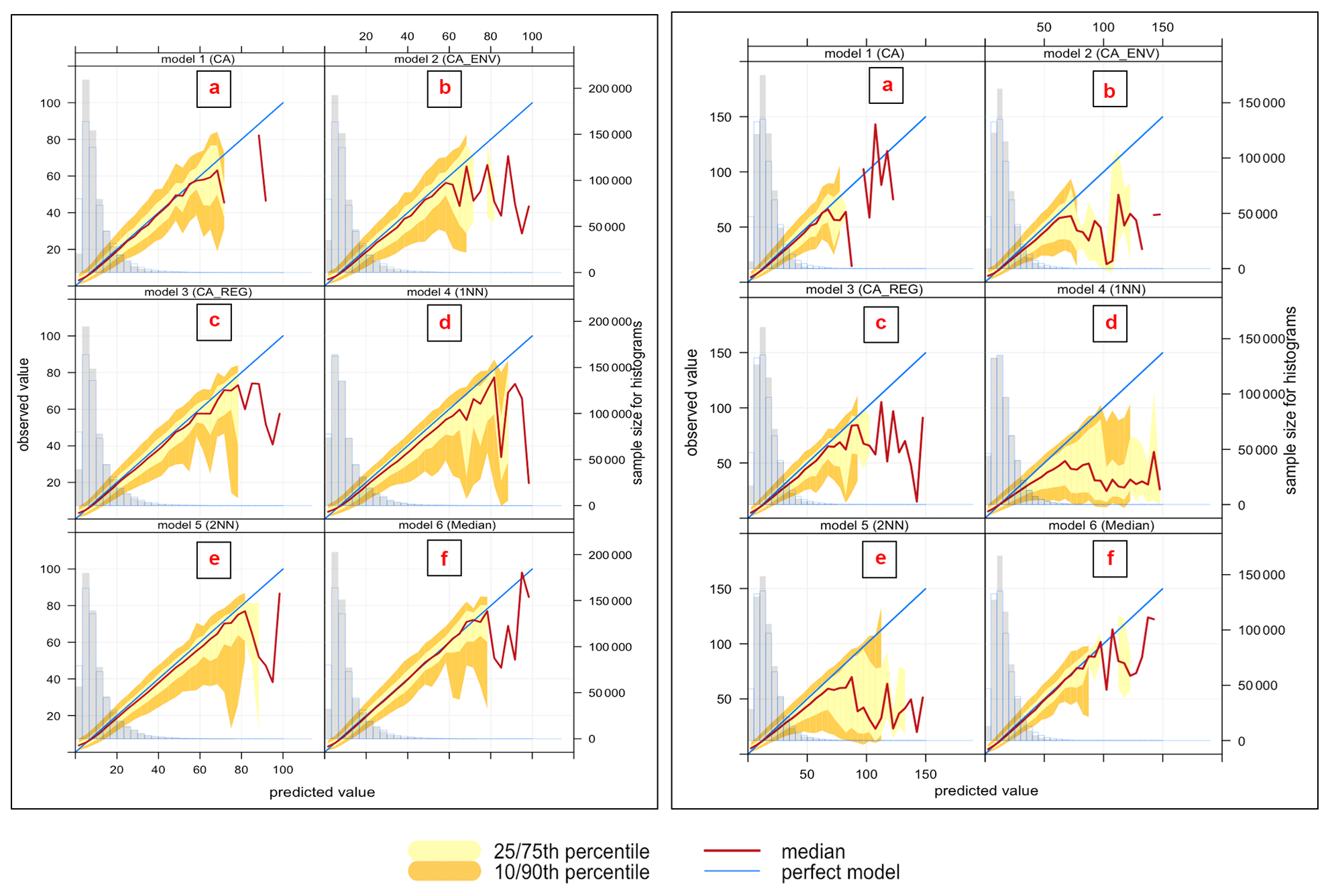
Figure 3Conditional quantile plot of modelled and observed pollutant concentrations of PM2.5 (left plot) and PM10 (right plot) for proposed imputation models: (a) model 1 (CA), (b) model 2 (CA+ENV), (c) model 3 (CA+REG), (d) model 4 (1NN), (e) model 5 (2NN), (f) model 6 (Median).
In Fig. 2 (left), the O3 models show that most modelled concentrations match the observations well for a wide range of values. The histograms indicate underestimation in general at the extreme low and high concentrations. In general, the cluster and Median imputation methods (i.e. that use averaging) will tend to struggle to reproduce the lowest and highest concentrations since they take an average approach. Moreover, the highest concentrations are typically limited to relatively few data points. The cases of high ozone concentrations typically occur during specific meteorological conditions and are episodic in nature, and there may be small differences in timings of the peak concentrations at different sites. Very low ozone concentrations are likely to occur at specific sites (near roads where emissions of nitric oxide are large) and therefore may not be reproduced in the models which take a cluster average or where a nearest-neighbour site is not a similar type of site.
Model 6 (Median) (panel f) has the best performance, as indicated by an overlapping median line with the blue line. This model has the lowest mean bias and the highest degree of agreement, as indicated by the narrow spread of the modelled concentration quantile intervals.
In the same figure (right), NO2 models show different behaviours from this analysis. Even though the statistical analysis shows that model 2 (CA+ENV) (panel b) gives the best performance, it is clear that in this model, the modelled concentrations tend to be lower than observations for most concentration levels (the medians are under the blue line), and the width of the 10th and 75th as well as the 10th and 90th percentiles is quite broad. The only advantage of using this model is its ability to capture a wide range of concentrations. Model 4 (1NN) (panel d) compared to other models can reproduce the higher concentrations (higher than 125 µg m−3) as it does not take an average approach. However, this model is positively biased (NMB = 0.095), which is shown by the departure of the median line from the blue one.
The variation between PM2.5 models in Fig. 3 (left) shows similar performance for the different models. The quantile intervals are wider within the area of high concentrations ≤60 µg m−3, and all models underestimate the high concentrations ≤80 µg m−3; note that these concentrations are very low-frequency events.
Model 6 (Median) (panel f) gives better performance, as indicated by the narrow spread of the modelled concentration quantile intervals and minimal bias, which is indicated by the overlaps between the red and blue lines compared to other models. Models for PM10 (right) show performance similar to PM2.5.
5.1.4 Model evaluation based on conditional quantile analysis and station environmental types
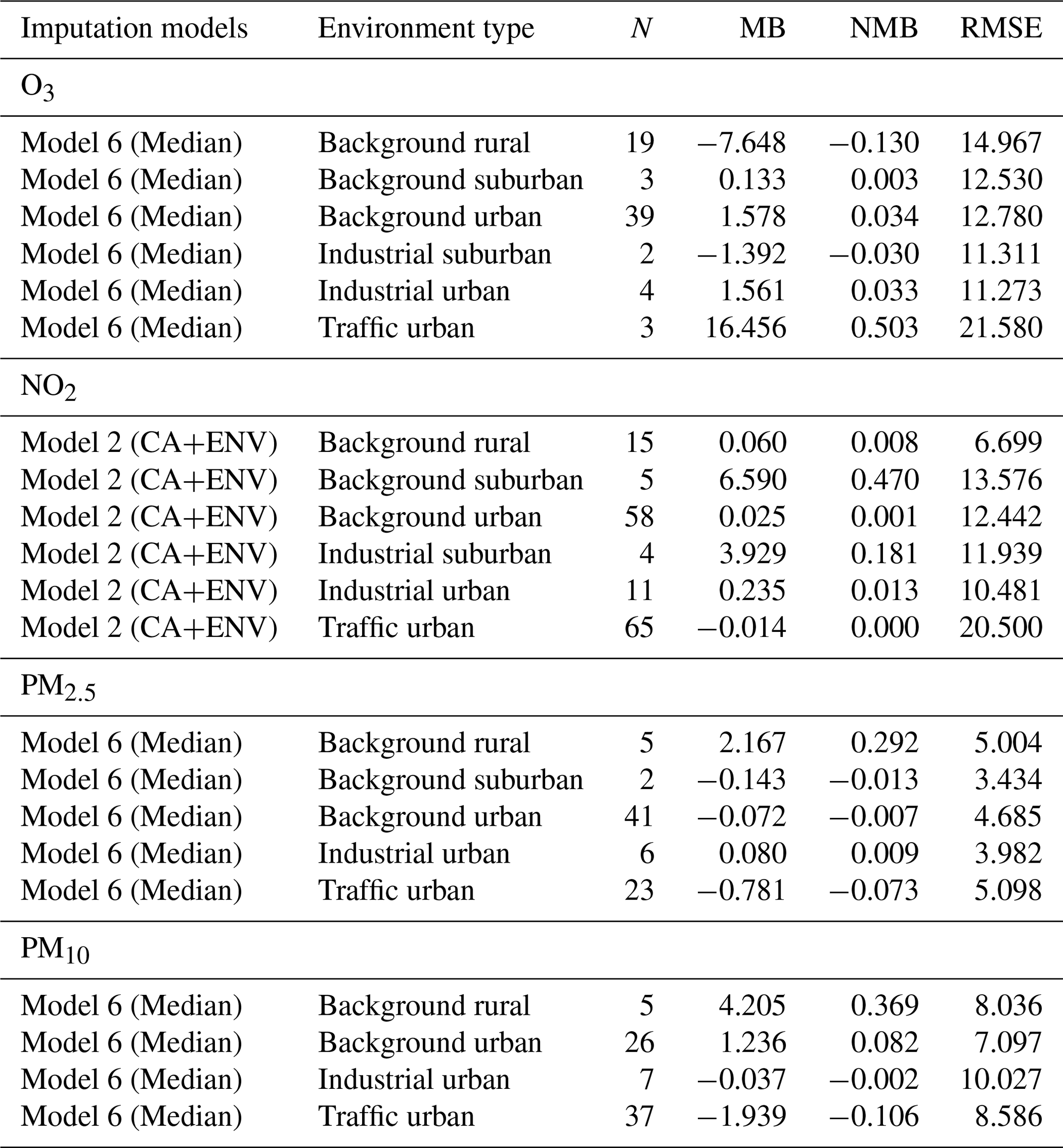
In this analysis, we focus on the performance of model 6 (Median) and model 2 (CA+ENV), as those performed best for the different pollutants in the previous section, but now we break down the analysis for the six environmental types (background rural, background urban, background suburban, and industrial urban, industrial suburban, and traffic urban) to which stations belong. Notice that a pollutant may or may not be measured in all stations and the number of stations of each type is different as shown in Table 2. We also use conditional quantiles to analyse our model's performance within each environmental type.
First, we show the monthly average concentrations for each pollutant under each environment type in our test dataset (year 2018) to understand the normal variation of the pollutant concentrations in different environment types. Figures 5, 7, 9, and 11 show conditional quantile plots by the environmental types for the selected models. Table 2 shows the statistical measures of performance also broken down by environment type.
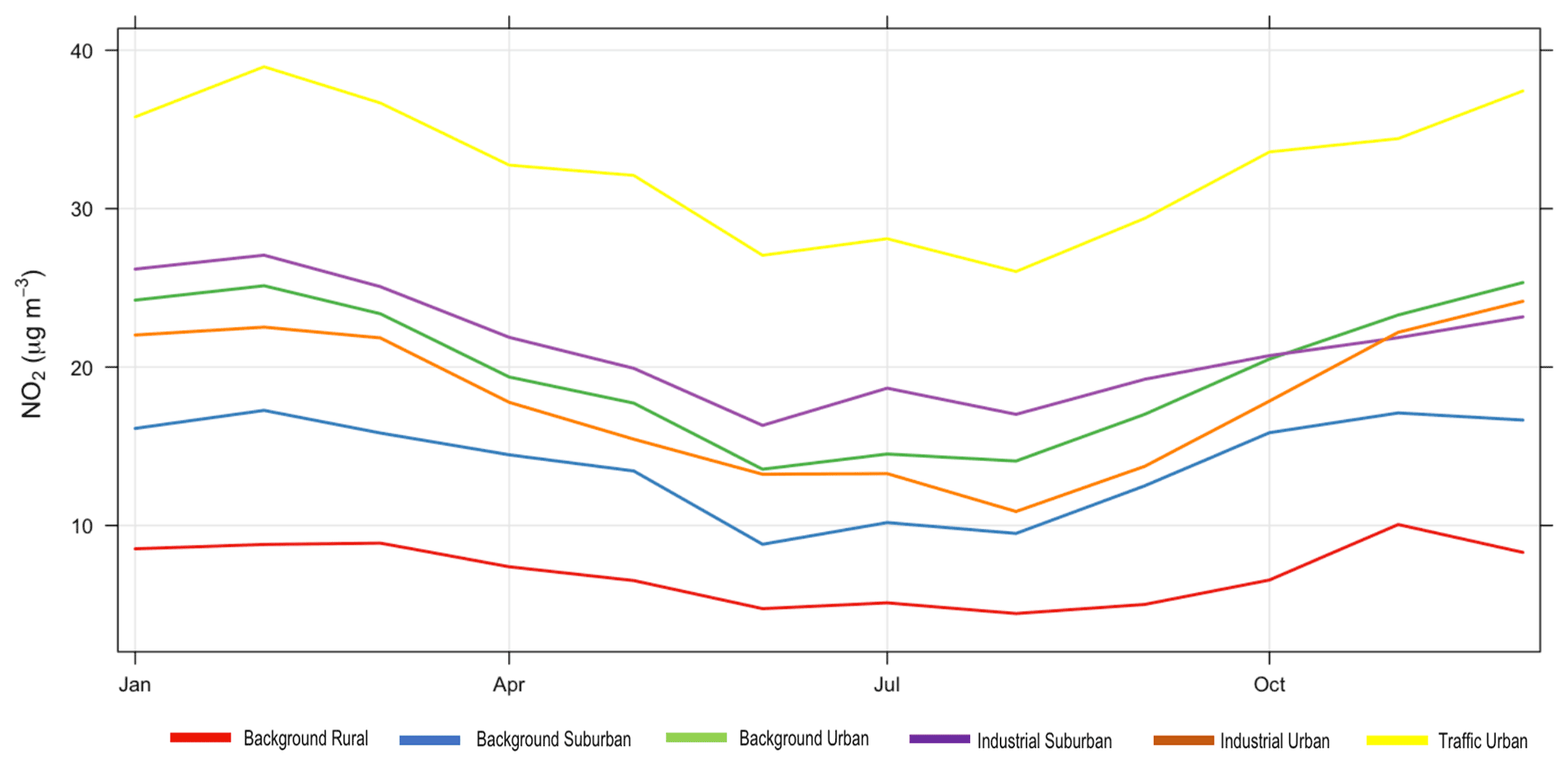
Figure 4Monthly average concentrations of observed NO2 for each environmental type for the year 2018.
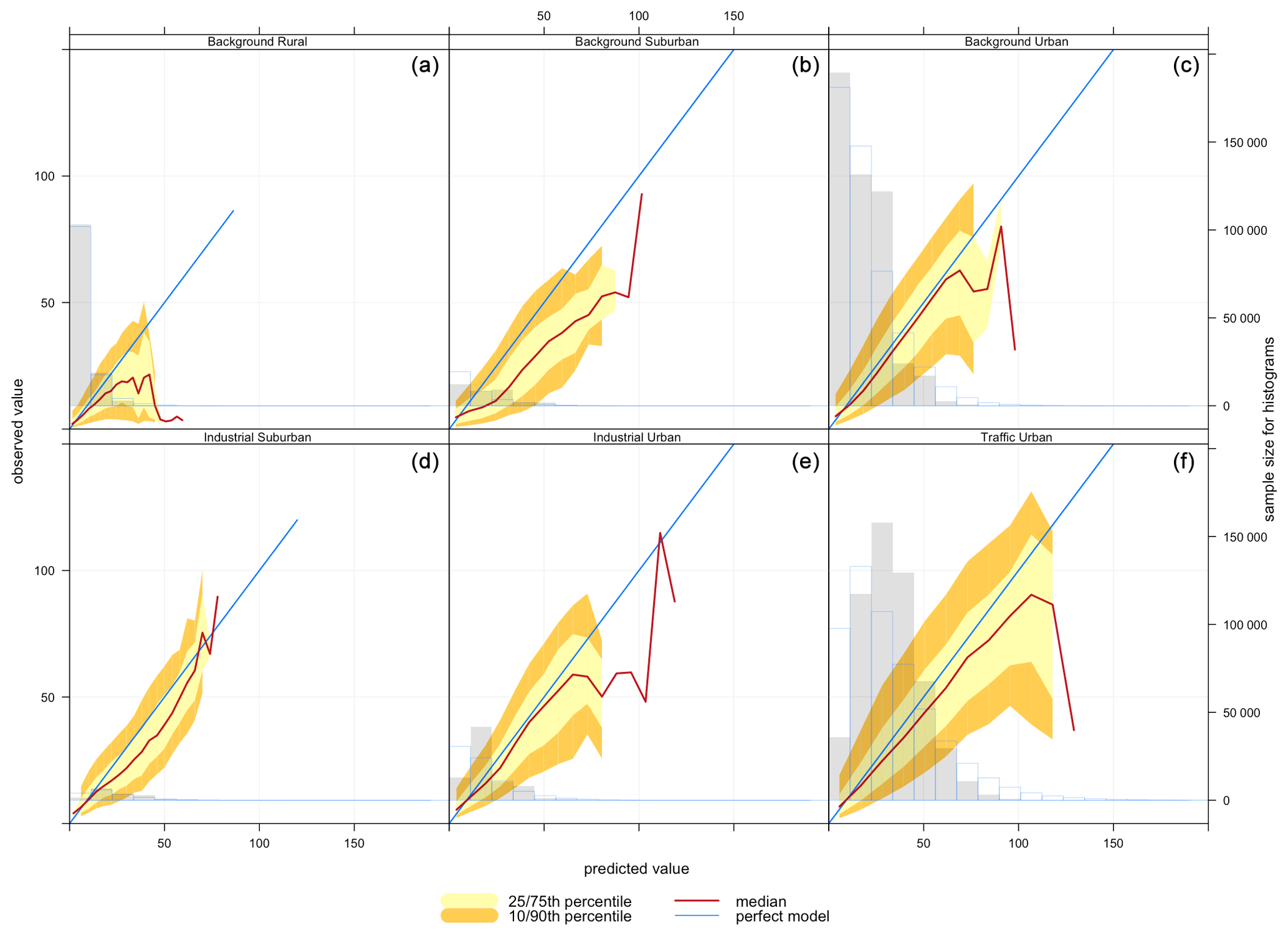
Figure 5Conditional quantile plot of modelled and observed pollutant concentrations of NO2 based on model 2 (CA+ENV) for all station environmental types: (a) background rural, (b) background suburban, (c) background urban, (d) industrial suburban, (e) industrial urban, and (f) traffic urban.
The most common sources of NO2 are roads; however, NO2 concentrations are influenced by traffic density, road locations, and meteorological conditions, which cause variation from one roadside location to another. Figure 4 shows that high NO2 concentrations are found at traffic urban followed by industrial suburban, then background urban sites, while the background rural sites have the lowest NO2 concentrations.
Figure 5 shows the conditional quantile plots by station type for NO2 imputation using model 2 (CA+ENV). Here, we see that modelled concentrations are higher than observed concentrations with all environmental types. This is confirmed by all the statistical model quality measures presented in Table 2, where we can observe a positive mean bias for NO2.
As NO2 distributions in general are skewed to the lower values and our selected model (model 2) (CA+ENV) is based on the average concentrations, the model performs better with lower concentrations.
From Table 2 based on model RMSE, the model's best performance is associated with background rural stations, while the worst performance is shown for traffic urban stations. Contrasting this with quantile plots, Fig. 5a shows that for background rural stations the histogram and the median line show better performance with lower concentrations (less than 30 µg m−3). On the other hand, for traffic urban stations (panel f), the quantile intervals are wider within the area of high concentrations (higher than 25 µg m−3), and the modelled concentrations tend to be lower than observed concentrations.
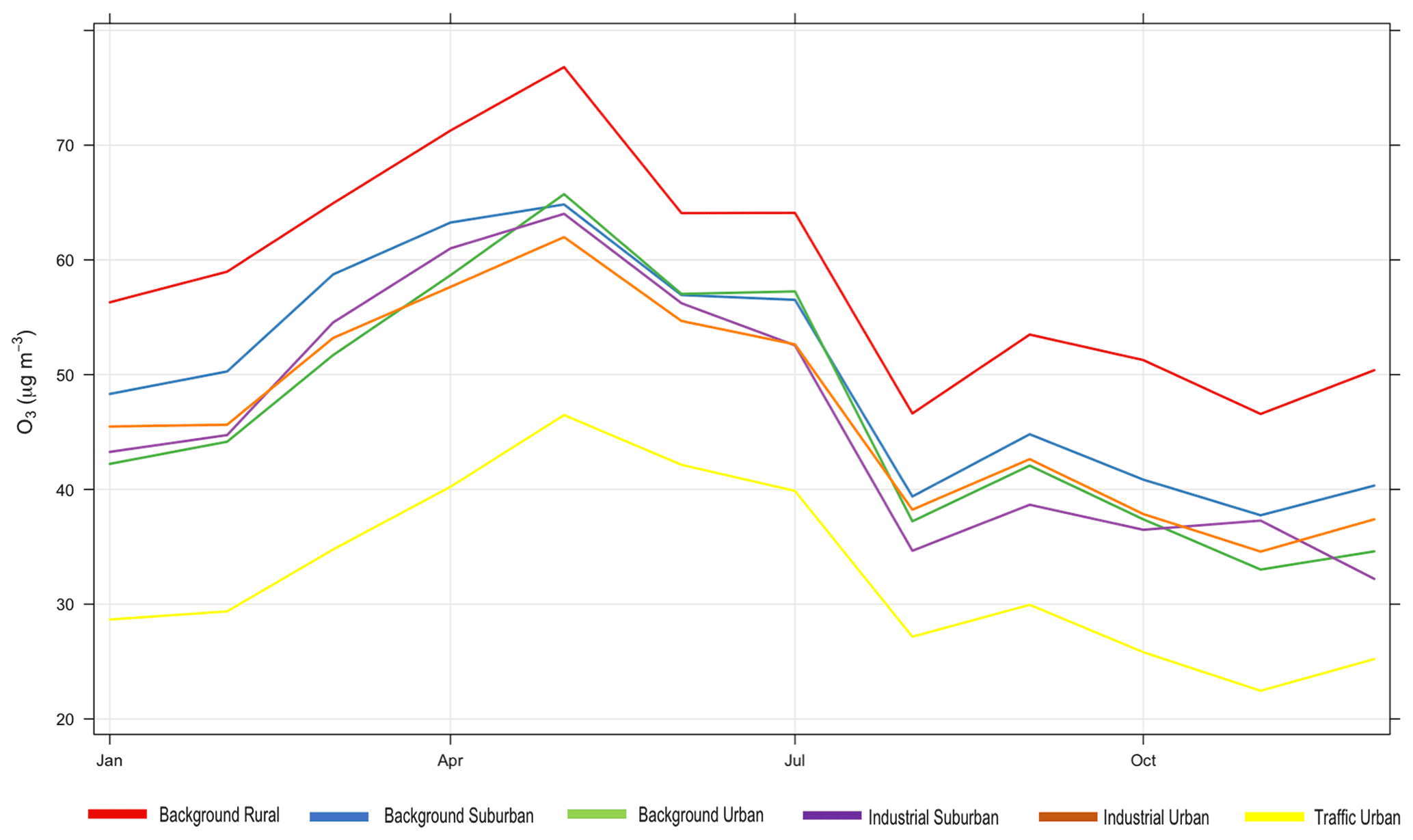
Figure 6Monthly average concentrations of observed O3 for each environmental type for the year 2018.
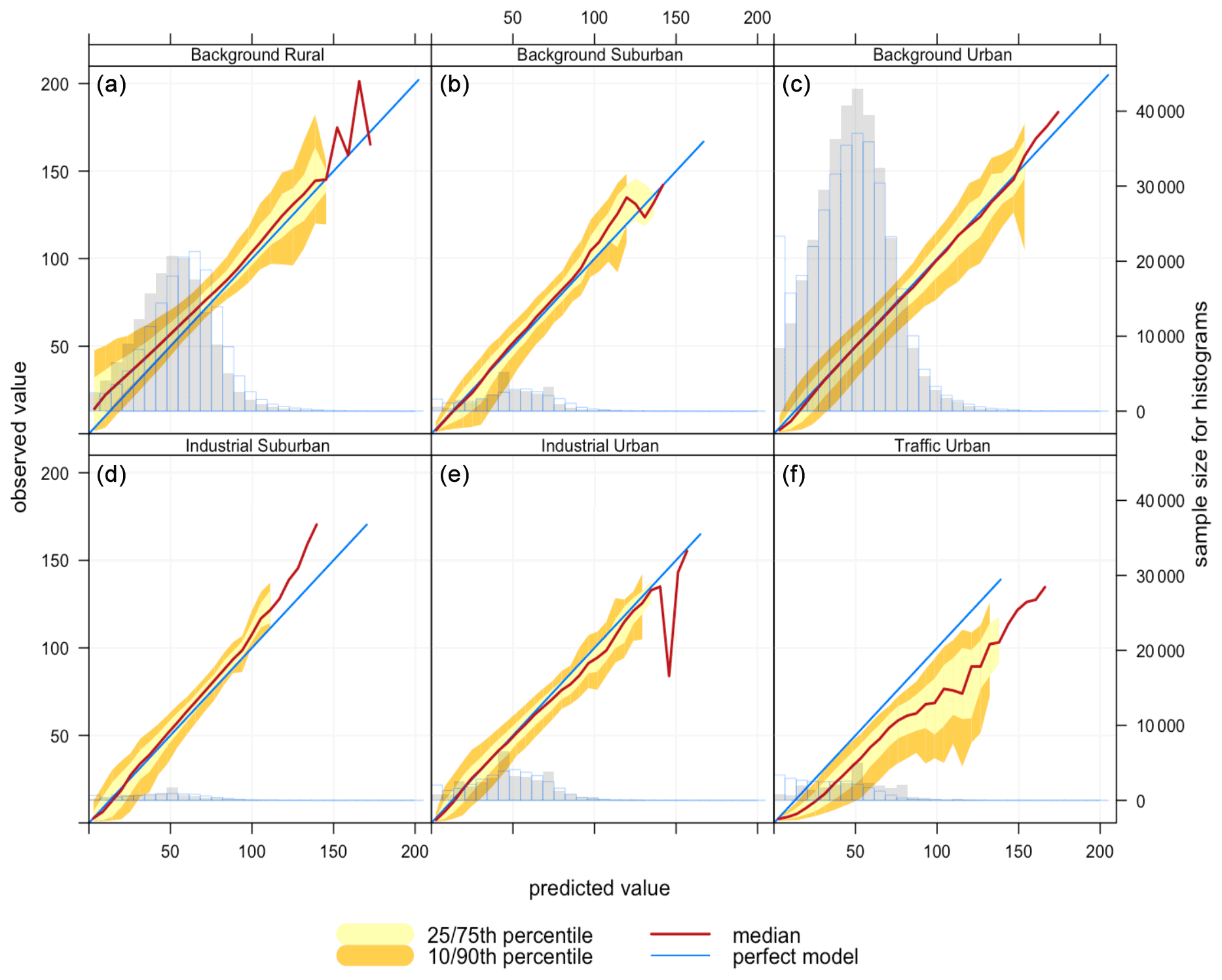
Figure 7Conditional quantile plot of modelled and observed pollutant concentrations of O3 based on model 6 (Median) for station environmental types: (a) background rural, (b) background suburban, (c) background urban, (d) industrial suburban, (e) industrial urban, and (f) traffic urban.
For O3, Fig. 6 shows the monthly average observed O3 concentrations in each environment type. From that we can see that ozone in all environment types follows a similar trend. However, background rural stations have the highest concentrations and traffic urban stations have the lowest, consistent with depletion of ozone due to rapid reaction with fresh emissions of nitric oxide from vehicles. Looking at model 6 (Median) performance in Table 2 based on the RMSE, the best model performance is associated with industrial urban stations, and its average performance is associated with background rural stations (those with higher concentrations in Fig. 6), while its worst performance is associated with traffic urban stations (those with lower concentrations in Fig. 6).
Conditional quantile analysis in Fig. 7 shows the performance of model 6 (Median) for imputing O3 for the six environmental types (panels a to f). The model shows similar performance for industrial suburban (panel d) and background rural stations (panel a). For both types, the model is negatively biased (see also Table 2), meaning that the modelled concentrations tend to be lower than observed concentrations (the median lines are above the blue lines).
The worst performance based on the RMSE is associated with traffic urban stations (panel f), which are the stations located at roadsides. With those stations, the modelled concentrations are higher than observed concentrations; i.e. the modelled histogram is shifted to the right. This is indicated by the model positive bias (0.503). The median line also extends beyond the blue line, which means that some modelled concentrations are much higher than observed measurements.
The best model performance is associated with industrial urban stations (panel e) according to the RMSE, even though background urban stations (panel c) appear to have the best performance by looking at the conditional quantile plots. The histogram in panel (c) indicates that the distributions of the observed and modelled concentrations tend to be closer to each other for higher concentrations. However, the model overestimates the average concentrations at these stations (between 25 and 70 µg m−3) and underestimates the very low concentrations.
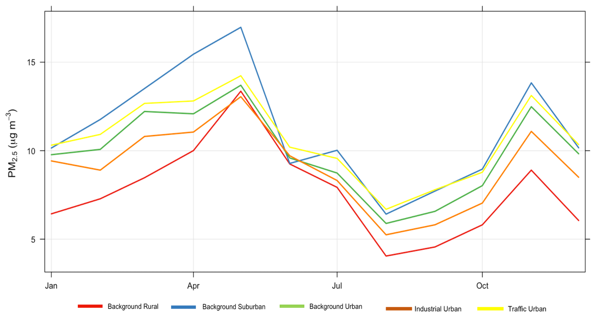
Figure 8Monthly average concentrations of observed PM2.5 for each environmental type for the year 2018.
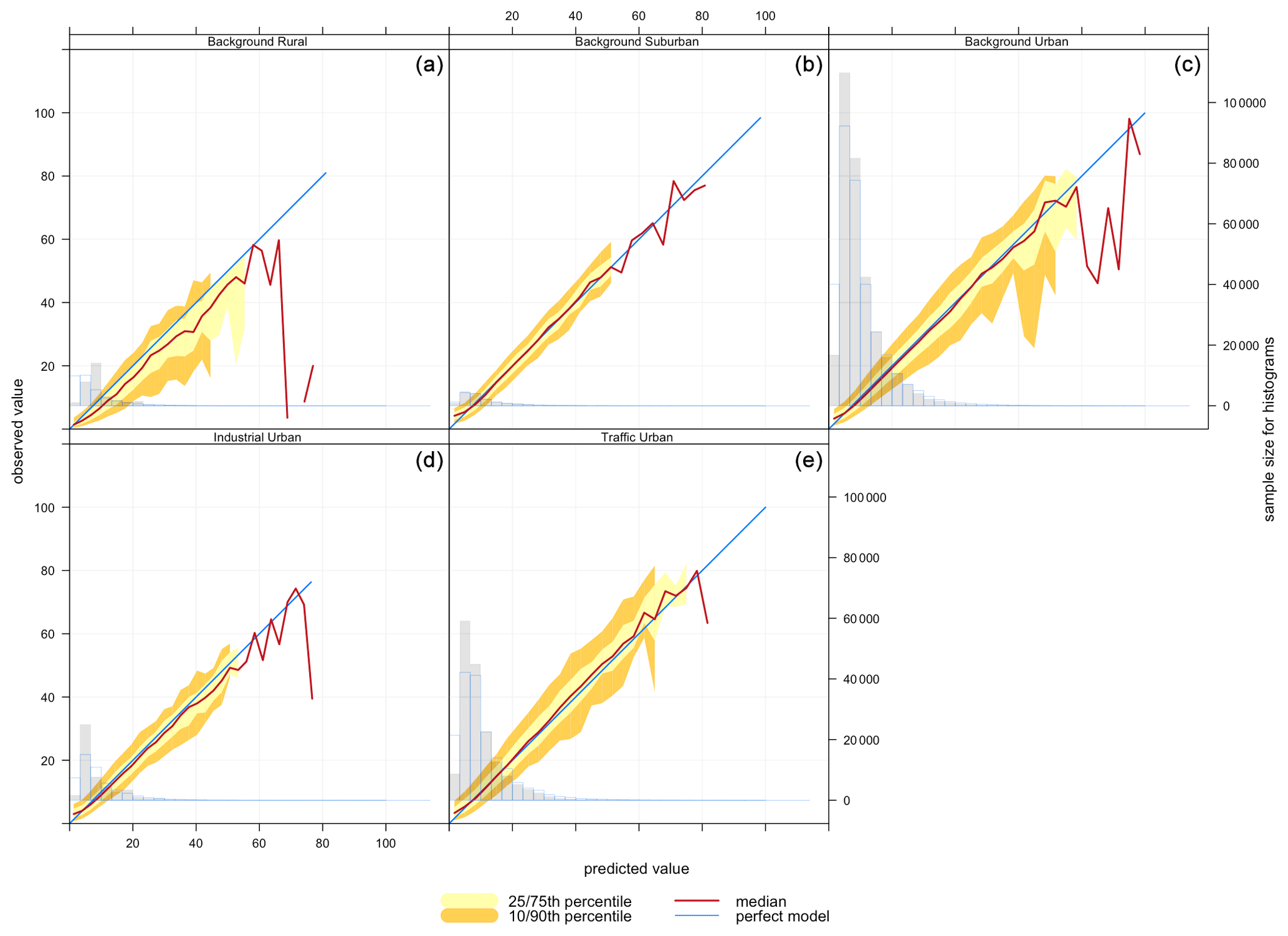
Figure 9Conditional quantile plot of modelled and observed pollutant concentrations of PM2.5 based on model 6 (Median) for station environmental types: (a) background rural, (b) background suburban, (c) background urban, (d) industrial suburban, (e) traffic urban.
Figure 8 shows that PM2.5 concentrations in rural areas are lower than those in suburban, urban background, and traffic urban areas. That is consistent with the model performance at these sites. Figure 9 shows corresponding conditional quantile plots by station types. Imputing PM2.5 concentrations using model 6 (Median) gives similar performance for the different station types. In general, the model underestimates the concentrations of PM2.5, especially for high concentration levels. Table 2 shows that the model underestimates high concentrations in suburban, urban background, and traffic urban areas, as indicated by the model negative biases, while it overestimates the concentrations at industrial urban and background rural sites. The model shows the worst performance for traffic urban (panel e), and this is also indicated by the highest RMSE (5.098) shown in Table 2. The model underestimates the concentrations at these stations, which is confirmed by the model bias (−0.073) in Table 2. On the other hand, the model's best performance is associated with background suburban sites (Fig. 9b), even though it underestimates PM2.5 concentrations with a mean bias of −0.013.
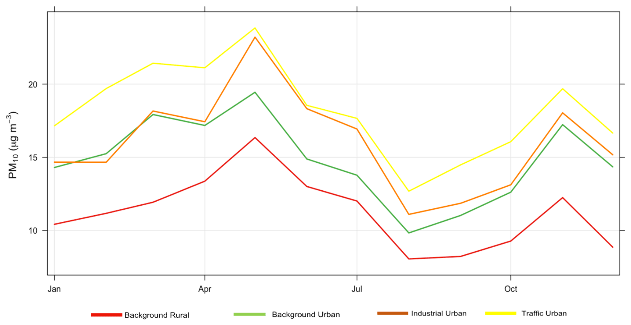
Figure 10Monthly average concentrations of observed PM10 for each environmental type for the year 2018.

Figure 11Conditional quantile plot of modelled and observed pollutant concentrations of PM10 based on model 6 (Median) for station environmental types: (a) background rural, (b) background urban, (c) industrial urban, (d) traffic urban.
Finally, PM10 levels in background rural and urban areas are lower than those in industrial and traffic urban areas as shown in Fig. 10. For PM10, imputation performance shown in Fig. 11 is similar for background urban and background rural sites (panels a and b). The model overestimates the concentrations of PM10 that are ≤10 µg m−3, while it underestimates the high concentrations of PM10 at industrial urban (slightly) and traffic urban sites (panels c and d). That is confirmed by the model mean bias at these sites (−0.002, −0.106) as shown in Table 2.
Table 2Performance of the hourly pollutant concentration imputation models using model 6 (Median) for O3, PM2.5, and PM10 and model 2 (CA+ENV) for NO2 based on statistical measures for all station environment types for all pollutants.
Next, we show some examples of our imputed TS compared to the real TS for each pollutant using the selected imputation models in some stations. The following examples in Figs. 12, 13, 14, and 15 show the observed and imputed hourly pollutant concentrations for the four pollutants using the selected imputation model that gave better imputation. We also apply the models for which there is a period of missing values in the observed concentrations to give some idea of how the models work for the whole TS, including when real values do not exist.
Figure 12 compares the observed hourly concentrations of PM2.5 (red) at London Eltham station for 1 to 15 January 2018 with imputed concentrations (black) using model 6 (Median). As we can see, the variation between the imputed and the real TS is very small and the imputed TS reproduces the trend very well, even though there is a period of missing concentrations within the observed TS (red). Similarly, Fig. 13 represents the observed hourly concentrations of PM10 (red) at Oxford St Ebbes station for the same period of time with imputed concentrations using model 6. We can see that model 6 underestimates the high concentrations and overestimates the very low concentrations of PM10 and PM2.5, as mentioned previously in the analysis in Sect. 5.1.3. However, there is still a good match of the trend.
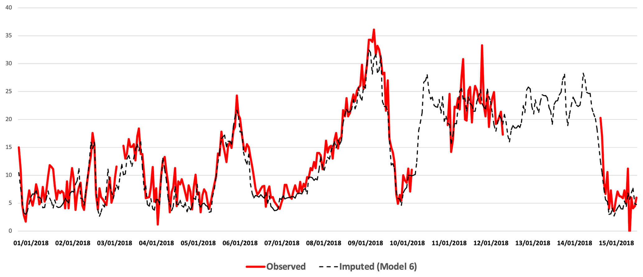
Figure 12Imputed (black) and real (red) TS comparison for PM2.5 at London Eltham station from 1 to 15 January 2018.
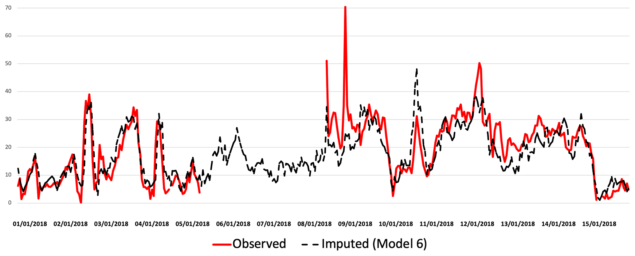
Figure 13Imputed (black) and real (red) TS comparison for PM10 at Oxford St Ebbes station from 1 to 15 January 2018.
Figure 14 shows a comparison of imputed (black) and observed (red) TS for NO2 concentrations at Birmingham Acocks Green station for the same period of time (1 to 15 January 2018), but produced by a different imputation model (model 3, CA+ENV) that gives better imputation than others for NO2. It is known that NO2 has greater spatial variability than other pollutants and it is very complex to impute; the variation between the imputed and the real TS is slightly higher when compared to the previous examples.
Figure 15 shows a comparison of the imputed (black) and observed (red) TS for O3 concentrations at Birmingham Acocks Green station for the period 16 to 23 January 2018 produced by model 6 (Median). The imputation underestimates the concentrations but represents the trends of high and low values.
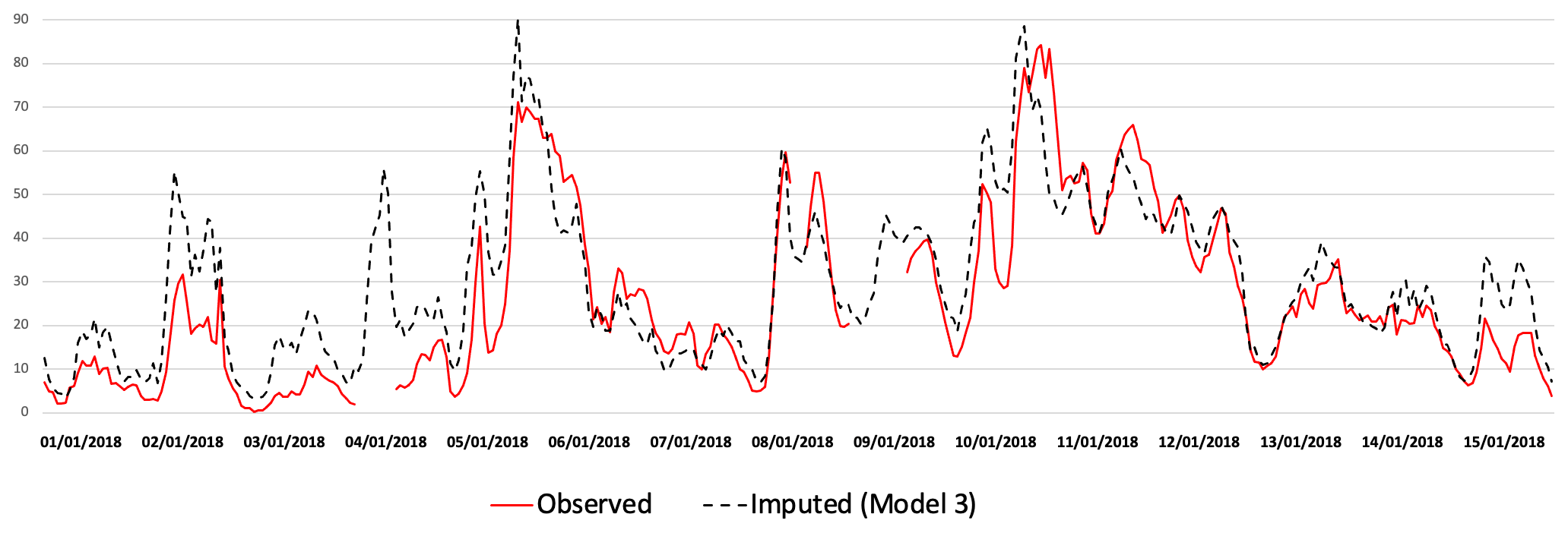
Figure 14Imputed (black) and real (red) TS comparison for NO2 at Birmingham Acocks Green station from 1 to 15 January 2018.
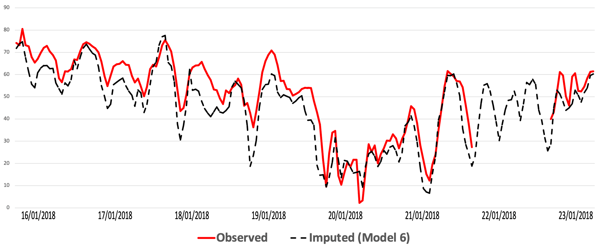
Figure 15Imputed (black) and real (red) TS comparison for O3 at Birmingham Acocks Green station from 16 to 23 January 2018.
5.2 Evaluating the imputed concentrations based on the Daily Air Quality Index (DAQI)
After imputing the measured pollutants in all the stations, we calculate the DAQI from the imputed data, as explained in Sect. 4.3. Then we compare it with the DAQI from the observed data to see our selected models' performances. The selected models are model 6 (Median) for O3, PM2.5, and PM10 and model 2 (CA+ENV) for NO2.
We compare the imputed DAQI with the observed DAQI based on RMSE and the number of days on which there are agreements and disagreements. The total number of days in our dataset is 60 955 d (167 stations ⋅ 365 d); there are 2212 d with missing observed DAQI (DAQI = 0) that have resulted from missing observations on those days. The total number of days to compare is 58 743 d.
In general, the total average RMSE from all days in all stations is 0.55. As the station type and the region may affect our imputation, Fig. 16 shows the average RMSE based on air quality regions in the UK (panel a) and station environmental types (panel b); the size of the circles represents the number of stations of each type. Panel (a) shows that stations classed as traffic urban are associated with the highest RMSE (0.62), while industrial suburban stations have the lowest RMSE (0.36). Panel (b) shows that the north-eastern region is associated with the lowest RMSE (0.44), while South Wales has the highest RMSE (0.74) between imputed and observed DAQI.
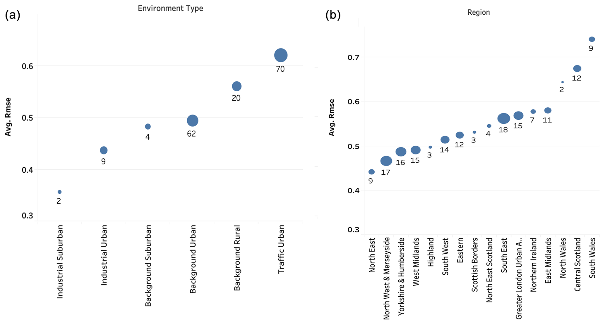
Figure 16The model performance based on DAQI RMSE: (a) the average of the RMSE based on station environmental types and (b) the average of the RMSE based on air quality regions.
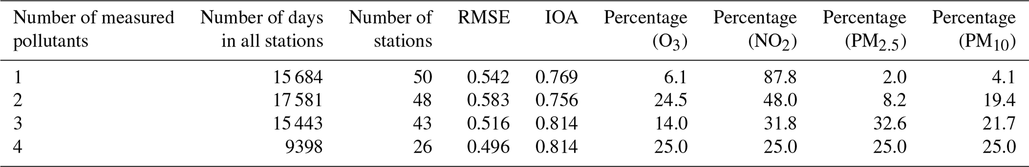
We also study the correlation between the number of measured pollutants in a station and the agreement between modelled and observed DAQI to see if the number of measured pollutants impacts our model's performance.
First, we classify stations based on the number of measured pollutants to stations that measured one, two, three, and all four pollutants, as shown in Table 3. Each row in this table represents one group. The second column is the total number of days with associated DAQI from all stations in each group. The RMSE and index of agreement (IOA) are the average of errors and the degree of agreement between observed and modelled DAQI from all stations in each group, then the percentage of each pollutant in each group. Based on this table, we find that stations that measure four pollutants have the lowest RMSE (0.506) and the highest (IOA) (0.806), while stations that measured one pollutant have the worst performance. The majority of stations with one pollutant are stations that measure NO2, with 87 % of the total number of stations in this group (50 stations).
Table 3Comparing observed and modelled DAQI based on the number of measured pollutants in stations.
We also compare the imputed and the observed DAQI based on the number of days on which the imputed DAQI agrees and disagrees with the observed DAQI. Table 4 shows those results and the percentage of time that these situations occurred, which means when agreement or disagreement is found for each DAQI. The total number of days on which the imputed DAQI agrees with the observed DAQI is 43 906 d (75 %), while there are 14 837 d (25 %) of disagreement. We classify the disagreement into two types: the imputed DAQI is higher or lower than the observed DAQI. We find that there are 10 916 d on which the imputed DAQI is lower than the observed DAQI and 3921 d on which the imputed DAQI is higher than the observed DAQI. In most cases, the imputed DAQI is lower than the observed DAQI, in accordance with our analysis of the imputation models that showed underestimation of the pollutant concentrations. From this table, we can see that the highest percentage of disagreement is 42.96 % of the total number of disagreements (14 837) when observed DAQI is 2 and imputed DAQI is 1, followed by 21.35 % of disagreement when observed DAQI is 3 and imputed DAQI is 2.
Table 4Number of days for which imputed DAQI agrees or disagrees with observed DAQI.

In this work, we evaluated our proposed models to impute missing pollutants in a station based on statistical and graphical model evaluation functions (Taylor diagrams and conditional quantile plots) that are designed to evaluate air pollution modelling. We found that the best imputation model based on statistical analysis is model 6 (Median) for O3, PM10, and PM2.5 and model 2 (CA+ENV) for NO2 imputation. The station environmental type plays an essential role with NO2 imputation because NO2 shows local patterns, as it is concentrated where it is emitted in urban areas and near the roadside. Adding to that, NO2 is shorter-lived than other pollutants and shows greater spatial variability, with concentrations being strongly influenced by the environment type (e.g. roadside, urban background, rural). This changes the NO2 concentrations from one location to another based on the environmental type (CenterForCities, 2020).
On the other hand, the graphical model evaluation functions showed these models' performance based on the distribution of the concentrations and the degree of agreement between imputed–modelled and observed concentrations. These functions help us to understand the relationship between the distributions of the observations and the model's performance. From the histograms in Figs. 2 and 3 we noted that the overall distributions of the observed concentrations of NO2, PM2.5, and PM10 are skewed to the lower values, while O3 has a more normal distribution. From these histograms, we also noticed that the distributions of the modelled O3 concentrations are shifted to lower values, while other pollutants' modelled concentrations are shifted to higher values. Hence, the model is not always able to reproduce the edges of the distribution correctly. The skewness in modelled values is mostly associated with model 1 (CA). As a consequence, this shows the greatest difference in skewness between the distributions of the observed and modelled values. However, model 1 (CA) in combination with others, as part of model 6 (Median), reduces the skewness in modelled values and generates better imputation, resulting in the lowest RMSE.
Model 6 (Median) is based on the median concentrations from stations with temporal and spatial similarity, so this model's expected performance is to underestimate the highest values and overestimate the lowest values with a normally distributed dataset. We found that the model performance can vary based on the environmental type and the nature of the pollutant, as shown in our analysis of model performance and DAQI RMSE.
Through our analysis, we also found that the variation of the model's performance with different environmental types is due to the pollutant behaviour and its emitted sources.
Model 6 (Median) performance with O3 imputation changes from one environmental type to another due to the ozone behaviour at these locations. As we know, ozone is not directly emitted into the air, but it is formed as a secondary pollutant by chemistry involving nitrogen oxides (NOx): the sum of NO2, nitric oxide (NO), and volatile organic compounds (VOCs) in the presence of sunlight (Diaz et al., 2020). This chemistry is non-linear, and newly emitted NO can react with O3, leading to reductions in O3 concentrations close to sources of NO (e.g. in urban areas and, in particular, close to roads). Consequently, ozone concentrations in urban areas are often lower than those in rural areas (Khan et al., 2017), as shown in Fig. 6.
Figure 7a shows that the model produces a distribution shifted to the left toward lower values, not capturing the ozone for rural areas that are associated with higher concentrations of O3. Similarly, industrial suburban stations (panel d) have a higher frequency of high concentrations (higher than 25 µg m−3), as shown in the histogram (panel d). Note that the majority of stations measuring O3 are background rural or background urban, with few stations in other categories. With traffic urban (panel f), for which the model performs the worst, some modelled concentrations are much higher than observed measurements. This lack of fit may be explained because ozone is suppressed by new emissions of NO close to sources (traffic), which reduces the amount of O3 at those station types.
From the same figure (panel c), as shown in the histogram for background urban stations, there is a high frequency of low concentrations (less than 10 µg m−3) at these stations that the model does not capture. This is consistent with the reaction of newly emitted NO from urban roadside that reduces the concentrations of ozone in urban areas. Based on the RMSE and NMB, the model is a middle-performing model. As shown in Table 2, the majority of stations measuring O3 belong to this type.
As we mentioned earlier, NO2 is short-lived, so it has large differences between sites near sources (roadside) and those further away. Based on the RMSE, model 2 (CA+ENV) performs better with lower NO2 concentrations than high values, and since these high NO2 values exist near traffic, the model performs the worst with traffic urban stations as shown in Fig. 5f. In contrast, the model's best performance is associated with background rural stations that have the lowest NO2 concentrations.
PM2.5 and PM10 have many varied sources, so for roads and industrial sites they can be associated with local sources, for example widespread primary sources (direct emissions) and diffused secondary sources (i.e. produced in the atmosphere following emissions of precursor gases). Whilst PM concentrations are often greater at roadsides (DEFRA LAQM, 2016), the particles can have lifetimes of several days in the atmosphere, meaning that they can be distributed widely. The larger particles are subject to greater loss via sedimentation, so PM2.5 is more evenly distributed than PM10 (National Statistics, 2020). This behaviour can also be observed with model 6 (Median) performance, for which there is less variation in the model performance under different environment types compared to the variation of NO2 and O3, as shown in Table 2.
We also observed that the distributions of NO2, PM2.5, and PM10 are skewed to lower concentrations, which impacts model performance at higher concentrations. All models perform worse for high concentrations of NO2, PM2.5, and PM10 than O3, as indicated by the width of the quantiles at high values shown in Figs. 2 and 3. Similarly, for lower concentrations, these models tend to perform better for NO2, PM2.5, and PM10 than for O3. However, our selected models (model 6, Median; model 2, CA+ENV) are able to overcome this impact slightly.
Our approach enables us to impute and/or estimate plausible concentrations of multiple pollutants at stations across the UK, and the modelled concentrations from the selected models correlated well with the observed concentrations. The performance of these models is very good, with a slight underestimation in model 6 (Median), especially with high concentrations. At the opposite end, model 2 (CA + ENV) slightly overestimates the NO2 concentrations due to the regional behaviour of this pollutant.
We also analysed the performance of these models based on the daily modelled concentrations under different weather types using Lamb weather types (LWTs), which are a synoptic classification of daily weather patterns across the UK (Lamb, 1972). We found that these models work equally well for all LWTs, so we did not include this analysis in this work.
In conclusion, MVTS clustering enables imputation even when no measurement is available for a given pollutant since the station can be allocated to a cluster based on the value of the other pollutants measured. Our proposed imputation models, model 6 (Median) for O3, PM10, and PM2.5 and model 2 (CA + ENV), give the best performance for imputing these pollutants. The advantage of these models is that they aggregate the spatial and temporal imputation. The spatial imputation is obtained from the nearest stations and the temporal imputation is obtained by MVTS clustering that clusters the stations based on similarity in time.
In our future work, we aim to improve our imputation by considering more information about the stations, such as station altitude and location in relation to the weather effects. We may also consider the correlation between pollutants in our imputation and include further analysis for the Daily Air Quality Index (DAQI), especially for those days when there is variation between imputed and observed DAQI. Finally, we need to study all possible uncertainty associated with this type of application, since the pollution level may change from year to year due to some pollution episodes caused by high temperature, wind, wildfire, or other factors.
Code and data are available at https://github.com/Wedad-O-A/Modelled-concentrations-/tree/v3.5.2 (last access: 27 October 2021) and https://doi.org/10.5281/zenodo.5602618 (Alahamade, 2021). Data at GitHub are generated by proposed imputation models. The inputs to these models are the original data collected from the DEFRA website (https://uk-air.defra.gov.uk/data/data_selector_service?show=auto&submit=Reset&f_limit_was=1, DEFRA, 2019).
The experimentation and initial draft were produced by WA as part of her PhD. IL and CER contributed ideas, co-supervised the PhD, and revised the draft papers. BDLI was the main supervisor for the work and contributed to the draft revisions.
The contact author has declared that neither they nor their co-authors have any competing interests.
Publisher's note: Copernicus Publications remains neutral with regard to jurisdictional claims in published maps and institutional affiliations.
We thank the anonymous referees for their useful suggestions and Salvatore Grimaldi for editing.
This paper was edited by Salvatore Grimaldi and reviewed by two anonymous referees.
Alahamade, W.: Wedad-O-A/Modelled-concentrations-: Modelled_Concentration_Air_Qaulity (v3.5.2), Zenodo [code and data set], https://doi.org/10.5281/zenodo.5602618, 2021. a
Alahamade, W., Lake, I., Reeves, C. E., and De La Iglesia, B.: Clustering Imputation for Air Pollution Data, in: International Conference on Hybrid Artificial Intelligence Systems, Lecture Notes in Computer Science, 585–597, https://doi.org/10.1007/978-3-030-61705-9_48, Springer, Cham, 2020. a, b
Alahamade, W., Lake, I., Reeves, C. E., and De La Iglesia, B.: A Multi-variate Time Series clustering approach based on Intermediate Fusion A case study in air pollution data imputation, Neurocomputing, in press, 2021. a, b, c
Austin, E., Coull, B. A., Zanobetti, A., and Koutrakis, P.: A framework to spatially cluster air pollution monitoring sites in US based on the PM2.5 composition, Environ. Int., 59, 244–254, 2013. a, b
Carbajal-Hernández, J. J., Sánchez-Fernández, L. P., Carrasco-Ochoa, J. A., and Martínez-Trinidad, J. F.: Assessment and prediction of air quality using fuzzy logic and autoregressive models, Atmos. Environ., 60, 37–50, 2012. a
Carslaw, D. C. and Ropkins, K.: Openair – an R package for air quality data analysis, Environ. Modell. Softw., 27, 52–61, 2012. a, b, c
CenterForCities: Cities Outlook 2020 – Air quality in UK cities, available at: https://www.centreforcities.org/publication/cities-outlook-2020/ (last access: 22 October 2021), 2020. a, b
DEFRA: Daily Air Quality Index implementation Report, available at: https://uk-air.defra.gov.uk/library/reports?report_id=750 (last access: 22 October 2021), 2013. a
DEFRA (Department for Environment, Food & Rural Affairs): Data Selector, available at: https://uk-air.defra.gov.uk/data/data_selector_service?show=auto&submit=Reset&f_limit_was=1, last access: 1 May 2019. a
DEFRA: About Air Pollution, https://uk-air.defra.gov.uk/air-pollution, last access: 22 October 2021. a, b, c
DEFRA LAQM: Public Health Sources and Effects of PM2.5, available at: https://laqm.defra.gov.uk/public-health/pm25.html (last access: 20 October 2021), 2016. a
Derwent, D., Fraser, A., Abbott, J., Jenkin, M., Willis P., and Murrells, T.: Report: Evaluating the Performance of Air Quality Models, Department for Environment, Food and Rural Affairs, London, 2010. a
Diaz, F. M., Khan, M. A. H., Shallcross, B., Shallcross, E. D., Vogt, U., and Shallcross, D. E.: Ozone Trends in the United Kingdom over the Last 30 Years, Atmosphere, 11, 534, https://doi.org/10.3390/atmos11050534, 2020. a
Di Bello, G., Lapenna, V., Macchiato, M., Satriano, C., Serio, C., and Tramutoli, V.: Parametric time series analysis of geoelectrical signals: an application to earthquake forecasting in Southern Italy, 1996. a
Du, S., Li, T., Yang, Y., and Horng, S.-J.: Multivariate time series forecasting via attention-based encoder–decoder framework, Neurocomputing, 388, 269–279, 2020. a
D'Urso, P., De Giovanni, L., and Massari, R.: Robust fuzzy clustering of multivariate time trajectories, Int. J. Approx. Reason., 99, 12–38, 2018. a
Fontes, C. H. and Budman, H.: A hybrid clustering approach for multivariate time series – a case study applied to failure analysis in a gas turbine, ISA T., 71, 513–529, 2017. a
Ignaccolo, R., Ghigo, S., and Giovenali, E.: Analysis of air quality monitoring networks by functional clustering, Environmetrics, 19, 672–686, 2008. a, b
Khan, M. A., Morris, W. C., Galloway, M., A. Shallcross, B. M., Percival, C. J., and Shallcross, D. E.: An Estimation of the Levels of Stabilized Criegee Intermediates in the UK Urban and Rural Atmosphere Using the Steady-State Approximation and the Potential Effects of These Intermediates on Tropospheric Oxidation Cycles, Int. J. Chem. Kinet., 49, 611–621, 2017. a
Lam, N. S.-N.: Spatial interpolation methods: a review, Am. Cartographer, 10, 129–150, 1983. a, b
Lamb, H. H.: British Isles weather types and a register of daily sequence of circulation patterns, 1861–1971, Geophysical Memoir 116, HMSO, London, 85 pp., 1972. a
Liao, T. W.: Clustering of time series data – a survey, Pattern Recogn., 38, 1857–1874, 2005. a
National Statistics: National Statistics Concentrations of Particulate Matter PM10 and PM25, available at: https://www.gov.uk/government/publications/air-quality-statistics/concentrations-of-particulate-matter-pm10-and-pm25 (last access: 22 October 2021), 2020. a
Sarda-Espinosa, A.: Package “dtwclust”, available at: http://cran.ma.imperial.ac.uk/web/packages/dtwclust/dtwclust.pdf (last access: 22 October 2021), 2017. a
Seto, S., Zhang, W., and Zhou, Y.: Multivariate time series classification using dynamic time warping template selection for human activity recognition, in: 2015 IEEE Symposium Series on Computational Intelligence, 1399–1406, IEEE, 2015. a
Taylor, K. E.: Summarizing multiple aspects of model performance in a single diagram, J. Geophys. Res.-Atmos., 106, 7183–7192, 2001. a
Tuysuzoglu, G., Birant, D., and Pala, A.: Majority Voting Based Multi-Task Clustering of Air Quality Monitoring Network in Turkey, Appl. Sci., 9, 1610, https://doi.org/10.3390/app9081610, 2019. a, b
Wickham, H., Averick, M., Bryan, J., Chang, W., D'Agostino McGowan, L., François, R., Grolemund, G., Hayes, A., Henry, L., Hester, J., Kuhn, M., Lin Pedersen, T., Miller, E., Milton Bache, S., Müller, K., Ooms, J., Robinson, D., Paige Seidel, D., Spinu, V., Takahashi, K., Vaughan, D., Wilke, C., Woo, K., and Yutani, H.: Package tidyverse, Easily Install and Load the Tidyverse, Journal of Open Source Software, 4, 1686, https://doi.org/10.21105/joss.01686, 2017. a
Zhou, P.-Y. and Chan, K. C.: A model-based multivariate time series clustering algorithm, in: Pacific-Asia Conference on Knowledge Discovery and Data Mining, 805–817, Springer, 2014. a