Swarm Langmuir probes' data quality validation and future improvements

Swarm is the European Space Agency (ESA)'s first Earth observation constellation mission, which was launched in 2013 to study the geomagnetic field and its temporal evolution. Two Langmuir probes aboard each of the three Swarm satellites provide in situ measurements of plasma parameters, which contribute to the study of the ionospheric plasma dynamics. To maintain a high data quality for scientific and technical applications, the Swarm products are continuously monitored and validated via science-oriented diagnostics. This paper presents an overview of the data quality of the Swarm Langmuir probes' measurements. The data quality is assessed by analysing short and long data segments, where the latter are selected to be sufficiently long enough to consider the impact of the solar activity. Langmuir probe data have been validated through comparison with numerical models, other satellite missions, and ground observations. Based on the outcomes from quality control and validation activities conducted by ESA, as well as scientific analysis and feedback provided by the user community, the Swarm products are regularly upgraded. In this paper, we discuss the data quality improvements introduced with the latest baseline, and how the data quality is influenced by the solar cycle. In particular, plasma measurements are more accurate in day-side regions during high solar activity, while electron temperature measurements are more reliable during night side at middle and low latitudes during low solar activity. The main anomalies affecting the Langmuir probe measurements are described, as well as possible improvements in the derived plasma parameters to be implemented in future baselines.

1 Introduction

Swarm is an Earth Observation mission of the European Space Agency (ESA) with the primary objective to measure Earth's magnetic field and its temporal variations, which enables investigations of, e.g. the core dynamics, geodynamo processes, and core–mantle interactions (Olsen et al., 2013). Further, the Swarm mission is devoted to characterize the ionospheric electric fields, currents, and other ionospheric plasma processes. The space segment consists of three identical satellites, which carry a diverse set of instruments to achieve the ambitious mission objectives: a vector field magnetometer (VFM) and an absolute scalar magnetometer (ASM) for collecting high-resolution magnetic field measurements, three star trackers for accurate attitude determination, a dual-frequency GPS receiver for precise orbit determination, an accelerometer to retrieve measurements of the satellite's non-gravitational acceleration, and an electric field instrument (EFI) composed of two Langmuir probes (LPs) and two thermal ion imagers (TIIs) for the plasma and electric field-related measurements. The three satellites were launched in 2013 into the same near-polar orbits. Shortly after launch, the satellites were manoeuvred into a constellation in which two satellites, Swarm A and Swarm C, fly side by side with 1.4^∘ separation in longitude at the Equator at an altitude of 462 km (initial altitude), and the third satellite, Swarm B, flies at a higher altitude of 511 km (initial altitude). Due to the difference in altitude, the orbital planes precess at different rates such that the angle between Swarm B's orbital plane and those of the other two satellites slowly change over time. In 2018, Swarm B's orbital plane was perpendicular to those of Swarm A and Swarm C, while by the end of 2021, Swarm B will be counter-rotating with respect to the lower-flying pair, which will result in a conjunction every 47 min.

With its plasma instrumentation (LP and TII, Knudsen et al., 2017), Swarm is an excellent mission to investigate and survey the ionosphere, its structure and dynamics. Recently, Swarm measurements brought more understanding of the space weather.

As reported by Archer et al. (2019), Swarm EFI measurements helped to advance the understanding of the auroral phenomenon known as “Steve”, which is visible as subauroral purple emission. By using Swarm LP electron density and temperature measurements this study demonstrates that Steve events are not only associated with intense subauroral ion drifts (MacDonald et al., 2018) but also with peaks of plasma temperatures and extremely low densities (Archer et al., 2019). The results presented in Archer et al. (2019) provided additional understanding of the Steve phenomena, expanding the knowledge needed for proper numerical simulations. More recently, De Michelis et al. (2021) discussed the possibility to use electron density measurements collected by LPs aboard Swarm, to derive a proxy for the ionospheric turbulence. This work suggests that, looking at the scaling features of the density fluctuations for different locations and geomagnetic activity levels, it is possible to distinguish two families of density fluctuations, one of which is most probably related to turbulent processes (De Michelis et al., 2021). Furthermore, the long time coverage of the Swarm mission offers the possibility to perform extended statistical analysis on the climatology of plasma irregularities via plasma-related measurements, as the in situ electron density data from the Swarm LP. The first global statistics obtained by in situ measurements of plasma variations observed by Swarm mission, confirmed the presence of three main regions of strong ionospheric irregularities: the magnetic Equator extending from post-sunset to early morning, the auroral ovals, and the polar caps (Jin et al., 2020). The long-term behaviour of density gradients and fluctuations has been studied by using Swarm data (Jin and Xiong, 2020), where LP density measurements are used to catch ionospheric structures and irregularities. This new statistical study describes phenomena already explored by past missions, but also reveals a new anomaly that is the persistence of strong density fluctuations in the southern polar cap during local summer (December solstice) (Jin and Xiong, 2020). The morning overshoot consists in a rapid increase of electron temperature in the early morning hours at low latitudes. Its dependence on geographic regions, local time, seasons and geomagnetic activity has been presented by Yang et al. (2020), by using electron temperature and density LP data at two different altitudes of the Swarm satellites, and ISS/FPMU (International Space Station/Floating Potential Measurement Unit) measurements (Coffey et al., 2008). Plasma density and temperature hemispherical asymmetries have been extensively investigated in ionospheric physics, and recently discussed by Hatch et al. (2020). In their study plasma density from both Swarm and CHAMP (Flury et al., 2006) measurements is used, demonstrating the importance of multi mission synergies and long mission life-time to statistically investigate ionospheric phenomena. For a comprehensive list of scientific results obtained with the support of the Swarm data, we refer to the Swarm webpage (European Space Agency, 2021b). It is worth to emphasize the role of LP plasma measurements in the recent ionospheric research field. As discussed above, LP data contributed to many scientific results advantaged by Swarm long-time mission coverage, multi-point in situ measurements as per Swarm spacecraft constellation, and continuously improved LP data quality. These studies demonstrated the scientific valence of LP measurements, and thus, the importance of an accurate monitoring of LP data with the scope to maintain high instrument performance and data processing accuracy.

The LPs are relatively simple instruments which are immersed into a plasma to measure electron density, N_e, and electron temperature, T_e. Owing to their simplicity, relatively small weight and low power consumption, LPs have been used on many satellite missions (Boyd, 1965; Abe and Oyama, 2013). Examples are Demeter (Lebreton et al., 2006), Rosetta (Eriksson et al., 2007), and Swarm (Knudsen et al., 2017). The science data derived from LPs aboard Swarm are part of the Level 1B (L1B) products and are obtained from the PLASMA operational processor. The LP data are available at both 2 and 1 Hz cadence. The algorithm of the PLASMA processor is described in the L1b Plasma Algorithm document (Buchert and Nilsson, 2018). To support the scientific research, the Swarm data products are continuously monitored for quality control (QC) and improved by the ESA/ESRIN Swarm Data Innovation and Science Cluster (DISC) data quality team. Also, users community feedback are essentials to improve the Swarm data product quality. Most of the feedback actually results in recommendations which are the drivers to elaborate and introduce improvements in the data processing algorithms (ESA, 2019). It is worth to specify that data quality is here intended as the goodness of the data product as output of a processing process. The data quality can be qualified by comparison with other dataset (in situ or ground measurement), validation with numerical or empirical models, or derived by statistical data analysis of the product itself. In our definition of data quality, if the data product is subject to a low level of errors as derived from statistical analysis or known issues, or/and has a high agreement with other dataset (model or spacecraft observations), then the quality of the data is considered good. In this paper the EFI-LP L1B data quality evolution introduced in the current baseline is described and the data quality status is statistically investigated. Known issues and future perspectives are discussed as well.

2 The Swarm Langmuir probes

The Swarm LPs have been described by Knudsen et al. (2017) including its “harmonic mode” with the sinusoidally modulated probe bias, in which the instrument is operated most of the times. Also the model equations that are assumed to determine the plasma density, the electron temperature and the spacecraft potential from the currents and admittances (which are the reciprocal of impedance) computed on board for given biases, are therein included. Complementing the description in Knudsen et al. (2017), we add here a detailed description of the LP instruments' functionalities and operational settings.

The two probes are mounted on the earthward edge of the ram panel as illustrated in Fig. 1. They are separated by 30 cm and located relatively close to the faceplate of the TII, which is also mounted on the ram panel. The LPs are expected to provide accurate and independent estimates of the spacecraft potential, which is in principle needed to process the TII data.

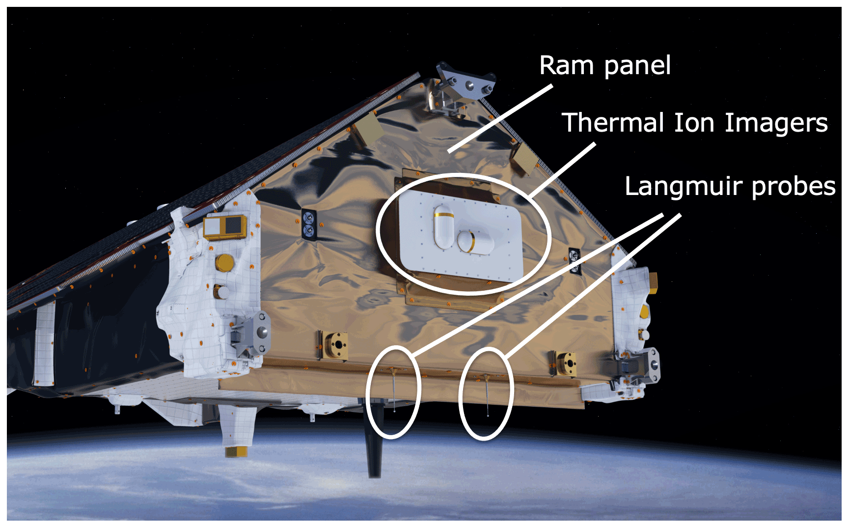
Figure 1 Location of the LPs below the ram panel. Image credits: ESA/ATG medialab.

The probes are also expected to provide plasma densities and electron temperatures over the entire range of signal magnitudes encountered along the orbit. Experimental results demonstrated that when the probes are immersed in the satellite plasma sheath, the estimation of spacecraft potential me by effected Wang et al. (2015), but so far the accuracy of current and density estimation from Swarm LP is not effected by this issue. The Swarm orbits will cover a limited range of altitudes from about 520 km shortly after launch to 250 km close to re-entry. But they sample practically all latitudes and local times, which results in a relatively large and dynamic signal range. Densities ranging from few hundreds cm⁻³ to several millions cm⁻³ can occur, representing more than 4 orders of magnitude. Avoiding an automatic gain control, which would potentially interfere with reliable and accurate current measurements, both probes are typically operated with fixed but different gains, called low and high gain (Knudsen et al., 2017). By electronically coupling a second shunt resistor in parallel, the mode is low gain which allows higher probe currents to be measured without ADC (analogue-to-digital converter) overflows. The term “gain” should be understood here rather as a sensitivity of the current measurement than an amplification. The ratio between high and low gain is about 50. High or low gain can be set by a telecommand from ground and usually one of the probes is in high and the other in low gain. Table 1 summarizes the differences between the probes and their gain operations.

Table 1 List of differences between the two LPs on each Swarm satellite. The probe position is defined with respect to the spacecraft coordinate system, where $\widehat{x}$ is along the fly direction, $\widehat{y}$ horizontally crosses the satellite toward local dusk, and $\widehat{z}$ points toward the Earth.

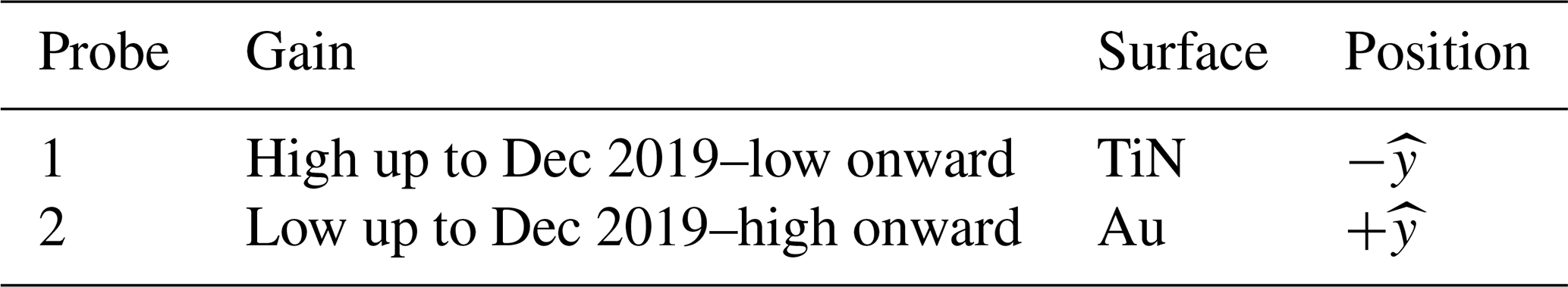
The surface material of one of the probes is titanium nitride (TiN), which had previously been used in several space missions, for example, Rosetta (Eriksson et al., 2007) and Demeter (Lebreton et al., 2006). Out of concern of the aggressive chemical reactivity of ionospheric oxygen (O), the other probe surface is made of gold-plated (Au) titanium (Ti), which is a novelty in space. It is known that Ti is very difficult to electroplate (e.g. ENS-Technology, 2022); however, a small company with experience in gold-plating jewellery made of titanium was given the contract. Testing before launch did not reveal any problems with the Au probes even after baking with temperatures of up to 300 ^∘C and after exposure to ultrasound. Both the nitration to TiN and the gold-plating are supposed to prevent strong oxidation of the Ti surface. Probably this would negatively affect the performance of the probe, because TiO is a relatively poor conductor. Presently, after more than 7 years in an O-dominated atmosphere, there are no conclusive indications in the in-orbit data that degradation in the form of serious oxidation of any of the probes has occurred, or that either of the two methods is preferable compared to the other one.

3 LP data processing

The L1B PLASMA processor, which is used to generate the LP data products, is organized according to the simple flowchart reported in Fig. 2. It uses as inputs the L1B products, containing position and velocity of the satellite, auxiliary data, and EFI-LP Level 0 (L0) data, to obtain three L1B and one Level 1A (L1A) data products. The auxiliary data contain information that support the Swarm data processing, such as physical constants, or instrumental calibration parameters obtained during ground tests. The L0 data contain raw measurements from each Swarm instrument and are essential to generate the L1 products. The EFI-LP L1A product (EFIX_LP_1A) contains information about the LP configuration, ion and electron currents in different regimes, and bias voltages. The L1B product LP_X_CA_1B delivers the LP calibration parameters derived for each probe by the L1B PLASMA processor. Finally, the EFIX_LP_1B and EFIXLPI_1B products provide the plasma parameters as density, electron temperature, plasma potential, together with the spacecraft position and the flags indicating a possible source of error for each data point. The EFIX_LP_1B are available at a 2 Hz sample rate. By simple linear interpolation of these products at full UTC second, the EFIXLPI_1B data product is obtained at 1 Hz sample rate. Also, the LPs operate in different modes. The “harmonic mode” (HM) consists of sinusoidal varying biases applied to the LPs. Each HM cycle lasts for 0.5 s, and during this time the HM currents and admittances are measured. To our knowledge, this method to obtain the current–voltage (I–V) characteristic of the space plasma is being used in orbit for the first time. The HM operates most of the time, while the classical “sweep mode” occurs every 128 s and lasts for 1 s. In sweep mode, the I–V curve is measured traditionally by scanning the probe bias over a range that stretches from a dominant ion current (at negative bias) to a saturated electron current (positive bias). Sweep mode data are not used in the L1B PLASMA processor but are separately analysed and provided as an additional “advanced” product. Furthermore, every 6 h, a calibration mode is activated and a calibration data packet is generated on board. These data are used for calibration purposes, and during the calibration mode, short data gaps are registered in L1B PLASMA products. The EFI-LP data products, and the other Swarm L1B products, are provided in daily files with a latency of 4 d. Detailed information on Swarm L1B processors and data products is provided by DTU (2019a, b). The Swarm products are freely accessible through the ESA dissemination server (European Space Agency, 2021a). The next two sections describe the recent data products evolution and data quality characterization.

Figure 2 Schema of the L1B PLASMA operational processor. The blue boxes on the left side represent the input files, the central yellow box represents the PLASMA processor, and the right-side boxes represent the processor outputs. In particular, the green box contains the EFI-LP L1B data products.

Table 2 Main differences between baseline 04 and baseline 05.

3.1 Evolution from product baseline 04 to 05

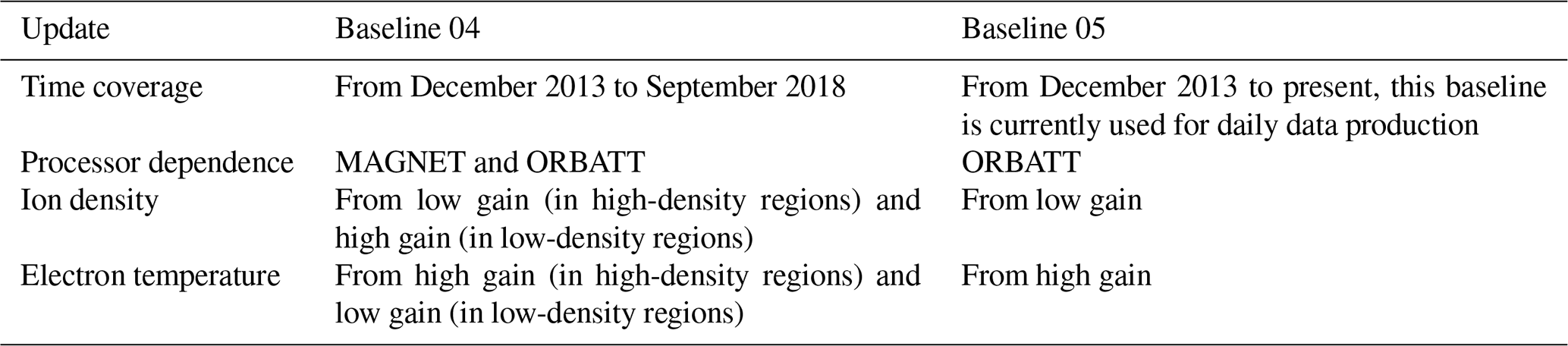
The product baseline is a number identifying the data that were generated in a consistent way, i.e. using the same algorithms and input parameters, and thus constitute a dataset. The product baseline is incremented when algorithm or input parameter upgrades lead to significant improvements in the data quality of the related products. The first PLASMA baseline went into operation in 2015 with the number 04. Before baseline 04, LP data were processed with a provisional processor by the Swedish Institute of Space Physics (IRF) (ESA, 2015). When the final version of the PLASMA processor was ready to be transferred into operation, it was deployed directly with baseline number 04 to be aligned with the other Swarm processor baselines. Thus, baselines lower than 04 are not available for EFI data products. Since September 2018, the PLASMA baseline has used the number 05. An updated version of this processor has been deployed in operation in February 2020 containing only minor evolution; thus, the baseline number remained unchanged. A complete description of all the evolution introduced with these processors is reported in the related technical notes (ESA, 2018, 2020b). In the following, we will discuss the major differences in PLASMA products between baselines 04 and 05, consisting of an updated electron temperature (T_e) computation from a high-gain probe, and the decoupling of the PLASMA processor from the MAGNET processor. Table 2 reports the main updates introduced in baseline 05, in comparison with baseline 04.

3.1.1 Electron temperature computation from the high-gain probe

Each of the two LPs aboard the Swarm satellites can be commanded to high or low gain. Typically, one probe is set to the low gain and the other one to the high gain. The LP product parameters can be estimated from each probe. In practice, the values often differ, which we suspect is because of the different probe gains. Many investigations are being carried out by the data quality team, in order to understand the nature of the difference between high- and low-gain measurements. Yet, a real conclusion has not been reached; thus we shelve the description of these studies for future work where a clear explanation may be reported.

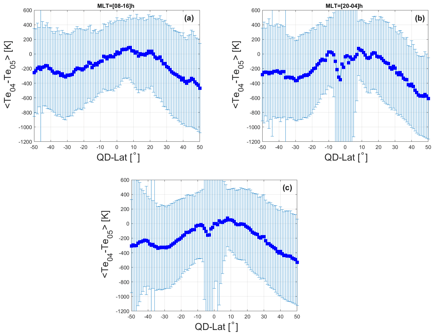
Figure 3 Difference between electron temperature T_e computed from baseline 04 ($T_{{\mathrm{e}}_{\mathrm{04}}}$) and 05 ($T_{{\mathrm{e}}_{\mathrm{05}}}$) as a function of quasi-dipole latitude, measured by Swarm A from 7 to 13 September 2018. Blue squares are the daily averages of each 1^∘ bin in latitude, while vertical bars represent the standard deviation. The figure shows the difference during (a) day-side, (b) night-side, and (c) full orbits.

The first analysis, preceding baseline 04, estimated the electron density N_e and electron temperature T_e from the high-gain probe for low densities or probe currents, from the low-gain probes for high densities or probe currents, and by blending the results from both probes for an intermediate range of density or probe current. This avoided sudden jumps which would be caused by switching the probes at threshold values. Typically the low-gain probe needs to be used at the dayside magnetic Equator because of very high density in the ionization anomaly, and the high-gain probe is more appropriate for other regions. In the commissioning phase, it became clear that the regularly occurring transition between probes produced unphysical variations of the estimated parameters even when smoothed by the intermediate blending. Therefore, the algorithm to estimate the density was changed to use the weaker ion current instead of the retarded and saturated electron currents. The ion current and admittance are always and very reliably measured by the high-gain probe. The density product is therefore rather an ion density product, though often designated still N_e. At Swarm altitudes, in the thermosphere and F region, the ion and electron densities are expected to be equal (only in the mesosphere and D region negatively charged ions and dust particles could cause N_e to be lower than the positive ion density). Also for T_e the blending of high- and low-gain estimates was eventually abandoned in order to avoid producing unphysical variations at transitions. This, however, has the drawback that especially in the ionization anomaly ADC overflow occurs in the high-gain-saturated electron current. This approach increased the number of T_e data with a flag for ADC overflow but with the benefit to have a dataset that can be better calibrated. The T_e from the low-gain probe is dropped in, with a flag value as warning. This modification has been introduced with baseline 05. The regions characterized by large plasma density are generally observed at equatorial and low latitudes. In particular, in correspondence to day-side equatorial crossings, it is possible to observe the typical double peak of the plasma density. This feature is related to the equatorial fountain effect characterizing the equatorial ionization anomaly (Kelley, 2009). Also, the ADC overflows are frequently observed at equatorial latitudes. Thus, to compare the measurements from baseline 04 (where high- and low-gain T_e measurements were blended together) and baseline 05 (where only high-gain measurements are used), it is worth considering the latitudinal variation. Figure 3 shows the differences between T_e obtained from baseline 04 ($T_{{\mathrm{e}}_{\mathrm{04}}}$) and baseline 05 ($T_{{\mathrm{e}}_{\mathrm{05}}}$) as a function of quasi-dipole (QD) latitude. The analysis is shown separately for day-side (Fig. 3a), night-side (Fig. 3b), and full (Fig. 3c) Swarm A orbits during 1 week in September 2018. The different phases of the orbits have been selected with respect to the magnetic local time (MLT). The analysis is limited to the latitudinal range to ± 50^∘ because at higher latitudes the electron temperature has a level of fluctuation too strong to obtain a meaningful comparison between $T_{{\mathrm{e}}_{\mathrm{04}}}$ and $T_{{\mathrm{e}}_{\mathrm{05}}}$. Figure 3 demonstrates that $T_{{\mathrm{e}}_{\mathrm{04}}}$ is on average larger that $T_{{\mathrm{e}}_{\mathrm{05}}}$ at higher latitudes. On the day side, the two baselines are comparable at equatorial latitudes (Fig. 3a), while the differences in this region are larger on the night side (Fig. 3b). In particular, the night side presents a negative peak between −10 and 10^∘ of QD latitude. Also, in Fig. 3c, we note a negative peak in correspondence to equatorial latitudes and a decrease for higher latitudes. Table 3 reports the average relative differences 〈 $\mathrm{\Delta }{T}_{\mathrm{e}}/T_{{\mathrm{e}}_{\mathrm{05}}}$ 〉 for each MLT range, where $\mathrm{\Delta }{T}_{\mathrm{e}}=T_{{\mathrm{e}}_{\mathrm{04}}}-T_{{\mathrm{e}}_{\mathrm{05}}}$. The results demonstrate that, on average, baseline 05 measures T_e, which is 5 %–10 % larger for the lower pair (Swarm A and C). This is a very good improvement, because it has been shown that the LP measurements of baseline 04, on average, underestimate the electron temperature with respect to ground measurements (Lomidze et al., 2018). Thus, the larger T_e measurements obtained with baseline 05 represent a better agreement with ground observations.

3.1.2 Decoupling between PLASMA and MAGNET processors

In the previous configuration related to baseline 04, the PLASMA processor had a dependence on the MAGNET and ORBATT processors. The ORBATT processor is fundamental for the L1B processing chain because it generates the L1B satellite ephemeris and attitude products, which are inputs for all the other processors. The MAGNET processor generates L1B magnetic measurement data products, which also contain the satellite position and attitude for convenience. The PLASMA processor needs as inputs the spacecraft position and velocity expressed in the Earth-fixed reference frame. In baseline 04, the spacecraft velocity was retrieved from the ORBATT processor, while the spacecraft position was retrieved from the MAGNET processor. Also, in baseline 04, magnetic measurements from MAGNET processor were needed to compute electrical field from TII measurements. This dependence on other processors implies that if one of those has a partial or total failure in producing the data products, then also the PLASMA processor fails. However, it was observed that the dependence on the MAGNET processor was not necessary, since the generation of the electrical field from TII measurements were removed from the PLASMA processor in baseline 05. Therefore, in the latest baseline, satellite position and attitude data can be directly retrieved from the ORBATT data products. As a consequence, with baseline 05, the PLASMA processor is decoupled from MAGNET, and it is now depending only on the ORBATT processor. This decoupling offered the opportunity to recover past data gaps that occurred because of MAGNET failures. In particular, with baseline 05, it was possible to recover the production of 4 d for Swarm A, 11 d for Swarm B, and 5 d for Swarm C. A full list of recovered data products is available in ESA (2020a). Even if it is a very small portion of data that has been recovered over more than 7 years of Swarm measurements, this still represents an improvement introduced with respect to the older baseline 04. Finally, we note that the decoupling of PLASMA from the MAGNET processor has no impact on the LP data quality.

Table 3 Average relative difference between $T_{{\mathrm{e}}_{\mathrm{04}}}$ and $T_{{\mathrm{e}}_{\mathrm{05}}}$ for all the Swarm spacecraft for different MLT ranges. The results are obtained considering 1 week of data from 7 to 13 September 2018.

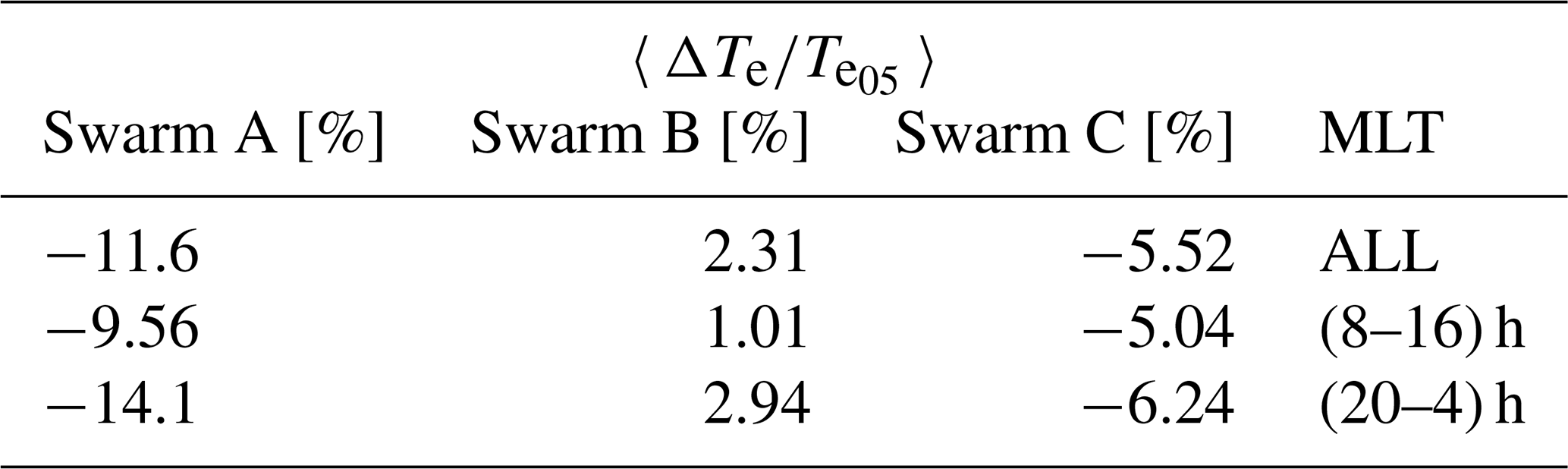
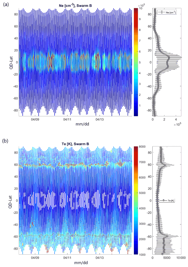
Figure 4 Plasma density (a) and electron temperature (b) measured aboard Swarm B between 8 and 15 March 2018, as a function of latitude in quasi-dipole coordinate and time. The vertical lateral panel shows the average (squares) and standard deviation (vertical bars) for each degree in latitude. During this period, the spacecraft was performing a noon–midnight orbit.

3.2 Baseline 05

Baseline 05 covers the data products from December 2013 to the present (this baseline is currently used for daily data production, and data coverage with baseline 05 will increase until a new baseline will be released). The LPs aboard Swarm can well capture the ionospheric variability in shorter intervals of time. Figure 4 shows the variation of plasma density and electron temperature as measured by Swarm B. Invalid measurements are removed in this figure. The missing data at equatorial latitudes in Fig. 4b are mainly due to ADC overflows, which generate invalid measurements. An interesting feature, that is worth noticing, is the typical double peak of the electron density at equatorial latitudes. This effect is related to the equatorial electrojet fountain (Kelley, 2009), and it is well visible in the Swarm measurements. In fact, at mid–low latitudes the density is higher, showing two peaks at around ± 10^∘ of QD latitude and slightly lower values at around 0^∘. At higher latitudes, the density is lower again. The electron temperature instead presents a different feature showing lower values at midlatitudes and low latitudes, and higher values at higher latitudes. This is another typical characteristic of ionospheric plasma (Kelley, 2009).

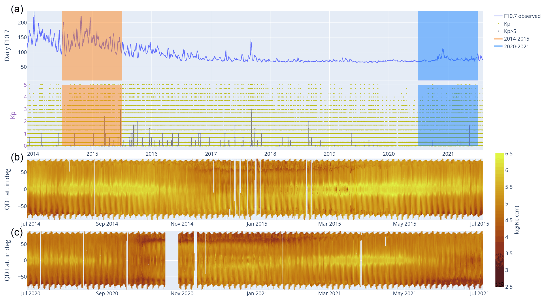
Figure 5 Overview of F10.7 cm and Kp indices over the ≈ 7 years of Swarm in orbit. The top panel (a) shows the 10.7 cm radio flux; the panel below (b) shows the Kp index. The bottom panels (c) show, with a logarithmic colour scale, the plasma density measured by Swarm A in ascending orbits for two representative time intervals of 1-year duration, July 2014–June 2015 and July 2020–July 2021. Time is on the x axis; the quasi-dipole latitude is on the y axis. The highest densities occur typically near the magnetic Equator on the day side, associated with the equatorial ionization anomaly. Very low densities are typically seen in the night-side midlatitude trough and around the winter polar cap.

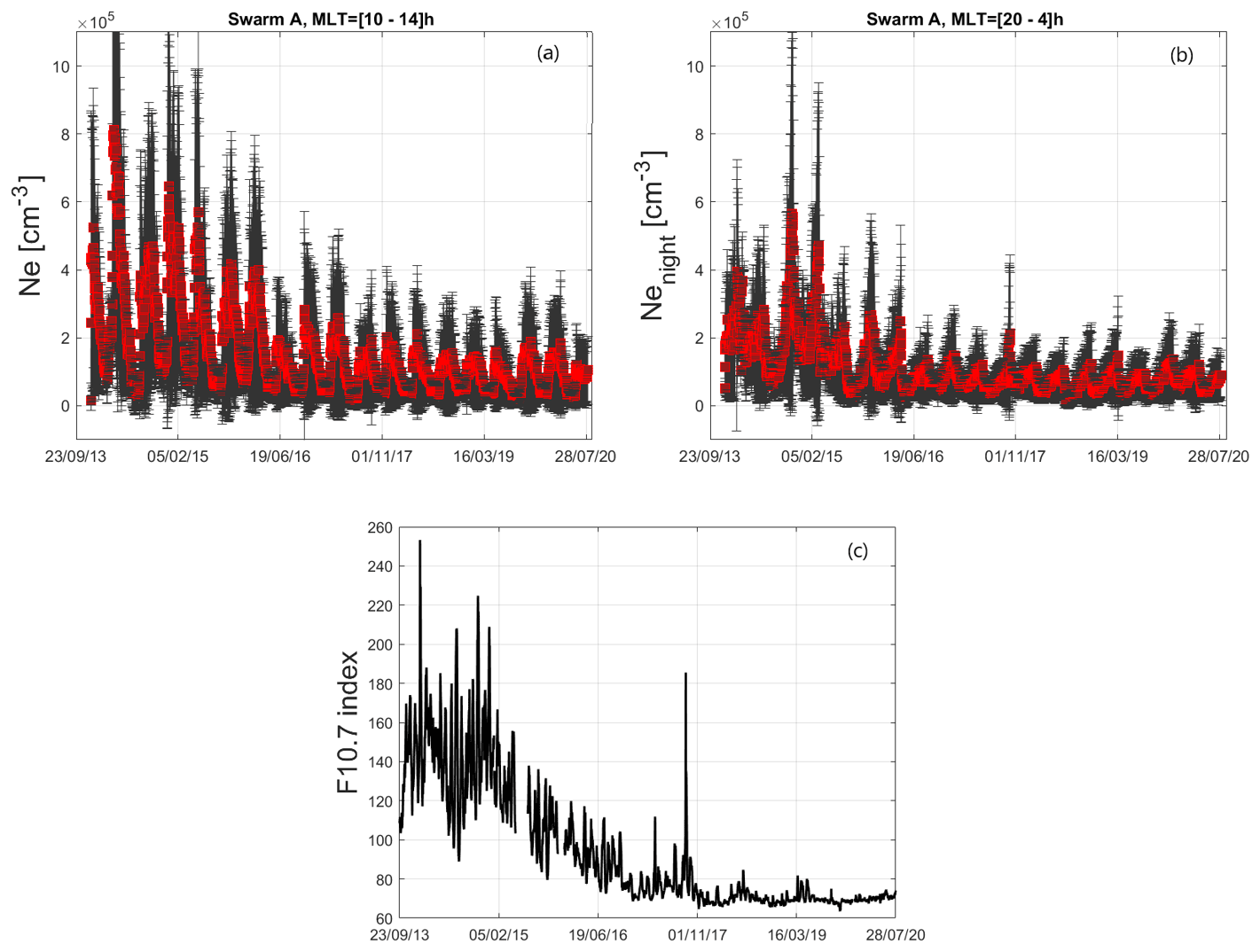
Figure 6 Orbital averages of the electron density variation (red squares) with standard deviations (vertical bars) during (a) ascending and (b) descending orbit phases, observed by Swarm A from December 2013 to July 2020. Panel (c) displays the F10.7 index in solar flux units for the same period. Similar results are obtained also for Swarm B and C (not shown).

During more than 7 years in orbit, the Swarm measurements span more than half of a solar cycle. Figure 5 shows the F10.7 index as an indicator of the solar activity, and the Kp index as an indicator of geomagnetic activity. The regions highlighted in orange represent the years when Swarm is in orbit. Such a long temporal coverage with Swarm measurements opens the opportunity to study the impact of solar activity on the ionosphere (Xiong et al., 2010) and to perform a long-term analysis of the ionospheric variations as well as multi-mission studies (Noja et al., 2013; Xiong et al., 2020). Here, we discuss the data quality variation of Swarm LP measurements with respect to the last solar cycle. The F10.7 index is used as reference for the solar activity (Covington, 1947, 1948; Tapping, 2013). The F10.7 index is a proxy for the solar extreme ultraviolet (EUV) flux, which is the dominating source of ionization, molecular dissociation, and heat in the thermosphere–ionosphere (see, for example, Liu and Chen, 2009; Vaishnav et al., 2019). Figure 6 shows the average plasma density variation from December 2013 to July 2020 as measured by Swarm A, separately for the ascending and descending orbit phases in Fig. 6a and b, respectively. Figure 6c shows the F10.7 index for the same interval of time. The density profile shows a high correlation with the F10.7 index. The solar radiation is the fundamental driver of density and temperature variations in the ionosphere (Prölss, 2004; Kelley, 2009). An example is the different characteristics of ionospheric plasma on the day and night sides, the latter having lower densities and higher temperatures (see, for example, Heelis and Maute, 2020, and references therein). Thus, the strong correlation between the F10.7 index and Swarm density measurements reported in Fig. 6, which is related to the ionospheric processes driven by the solar activity, represents additional evidence of the quality of the Swarm data.

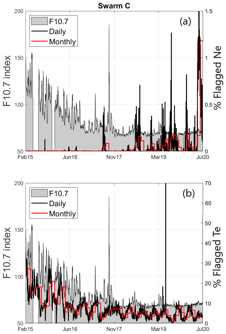
Figure 7 Daily (black lines) and monthly (red lines) percentage of invalid measurements (right axis) of (a) plasma density and (b) electron temperature measured by Swarm C from February 2015 to July 2020. The grey area in the panels represents the F10.7 index (left axis) in solar flux units in the same interval of time.

Each LP data point is associated with a flag indicating the instrument performance and settings, together with the source of possible errors. For more information on the flag, we refer the reader to Sect. 6.8 of DTU (2019b). The percentage of measurements that are flagged as invalid is a useful proxy for the data quality and instrument performance. A larger percentage of invalid measurements obviously indicates a poorer data quality. Figure 7 reports the daily and monthly percentages of invalid measurements from the beginning of the mission up to July 2020, for Swarm C. The results are reported for the plasma density and electron temperature in Fig. 7a and b, respectively. The shadowed area in the panels represents the F10.7 index variation in the same period. In Fig. 7b, we observe a common trend in the percentage of invalid measurements of electron temperature T_e and the F10.7 index, whereas the opposite trend is visible for the percentage of invalid measurements of plasma density in Fig. 7a. These trends are similarly observed for all three Swarm satellites. During the solar minimum, the plasma density decreases, as also shown in Fig. 6. In particular, the LP-derived plasma density is negative more frequently during the solar minimum. This feature is reflected in Fig. 7a by a larger number of invalid derived density data at lower F10.7 index values. During periods of stronger solar activity, we observe ADC overflows more frequently, which generate invalid T_e measurements. This feature is represented in Fig. 7b by a larger number of invalid T_e measurements at a lower F10.7 index. The geographical location and temporal variation in the occurrence of the invalid measurements are very useful to the Swarm EFI-LP team to study the instrument performance and to detect possible anomalies in the LP measurements.

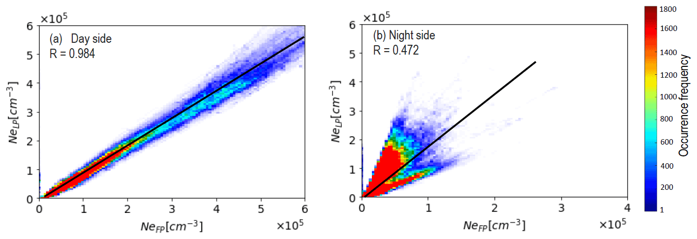
Figure 8 Comparison of the plasma density derived from the LP and FP on the (a) day side and the (b) night side as measured by Swarm C in February 2020. The black lines represent the linear fit obtained for the two datasets.

The plasma density can also be derived from the faceplate (FP) aboard Swarm as part of the TII instrument. The FP, similarly to a planar Langmuir probe (Oyama, 2015), measures the current with a cadence of 16 Hz. The electron density N_e is derived from FP current measurements only for certain orbits per day, namely when the TII is not active. The FP data and relative technical notes are available for all Swarm users (see IRF, 2017). A validation of LP density measurements can be performed by comparing the LP- and FP-derived densities. Figure 8 shows a scatter plot between density as measured by the LP and FP separately for the day (Fig. 8a) and night (Fig. 8b). We observe a very high correlation of 0.98 between the two datasets for the day side and a moderate correlation of 0.47 for the night side. The relative difference between the FP and LP density measurements, defined as $({N_{\mathrm{e}}}_{\text{FP}}-{N_{\mathrm{e}}}_{\text{LP}})/{N_{\mathrm{e}}}_{\text{LP}}$, is 19 % for the day side and 34 % for the night side, noting that the FP density measurements are generally higher than the LP density measurements. These results are in agreement with the recent study by Smirnov et al. (2021). In this context, it is worthwhile to emphasize that the LP processor algorithm needs to assume a certain ion composition. This assumption is that ionospheric plasma at Swarm height only contains O⁺ ions. The FP data processing is done independently of the plasma composition. However, a contribution of H⁺ to the plasma composition would cause thermal effects, because for H⁺ the satellite velocity is not much larger than the thermal velocity. This is so far not taken into account in the data processing. Thus, the discrepancy between the FP and LP measurements could be caused not only by noise at low densities but also by a contribution of H⁺ to the composition, in particular for the night side. Indeed, the electron density in nocturnal regions is lower compared to the day side, which is due to the weaker Sun illumination and consequently lower ionization on the night side and a larger number of molecular ions (Kelley, 2009; Heelis and Maute, 2020). The comparison between the FP and LP density measurements demonstrates that the two datasets are in good agreement in day-side regions. The results also show that the L1b PLASMA algorithm can be further improved by taking the difference in the ion composition between the day and night sides into account. Possible ways to improve the plasma density computation are under investigation and will be included in future baselines.

4 Known issues and future plans

The Swarm LP measurements have a high value for scientific investigations. However, few anomalies affect the LP measurements which are continuously monitored and investigated by the ESA data quality team and the scientific community. The source of these anomalies is only partially understood, which leaves open questions in both physical and instrumental domains. This section is dedicated to the description of the occurrence of one of these anomalies, namely the occurrence of extremely high values in the electron temperature measurements, which has a large impact on the data quality and scientific investigations. In addition, we describe the calibration of LP measurements, which will be introduced in the next baseline (06).

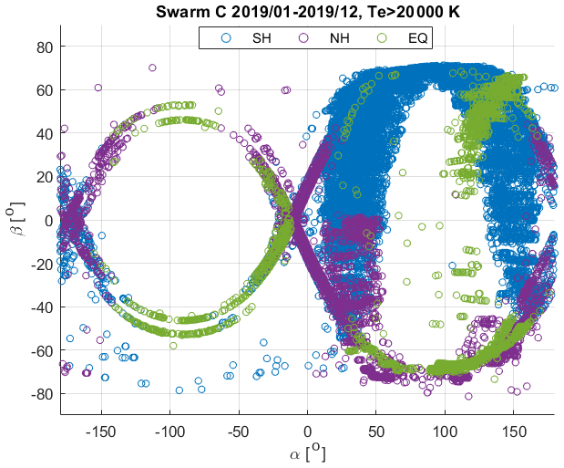
Figure 9 Electron temperature (T_e) extreme values as a function of solar elevation (α) and azimuth (β) angles as observed by Swarm C in 2019. Measurements located at latitudes between ± 50^∘ in QD coordinates are represented with green circles (EQ). Measurements at latitudes smaller than −50^∘ are represented by using blue (SH) circles. Purple circles (NH) denote measurements at latitudes larger than 50^∘.

4.1 Extreme T_e values

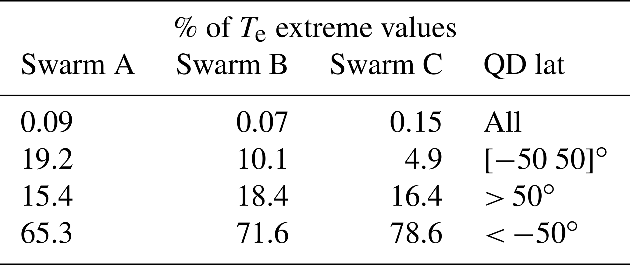
The ionospheric electron temperature typically ranges from a few hundred Kelvin during quiet periods at lower latitudes to a few thousand Kelvin during extreme events such as Steve auroral emissions (Archer et al., 2019), during which peaks of 8000 K were observed. However, the LP aboard Swarm satellites occasionally measures T_e values up to more than 20 000 K, which have to be considered “extreme”. Figure 9 reports the extreme T_e values that occurred in 2019 as a function of the solar elevation (α) and azimuth (β) angles with respect to the spacecraft. The extreme T_e values represent around 0.1 % of the data in 2019. In particular, about 19 % of the extreme T_e values are located between $\pm {\mathrm{50}}^{\circ }$ of QD latitude (green circles denoted EQ in the legend), 15 % are located at latitudes higher than 50^∘ (purple circles, NH in the legend), and 65 % are observed at latitudes below −50^∘ (blue circles, SH in the legend). It is worthwhile to notice that the distribution is more scattered for positive α values, i.e. when the Sun illuminates the spacecraft from the rear (anti-flight direction). On the opposite, we observe a more ordered distribution for negative α values, i.e. when the Sun shines on the front of the satellite. Similar results are obtained for all three Swarm satellites (not shown). This peculiar behaviour suggests that part of the T_e extreme values are probably related to instrumental disturbances possibly triggered by the Sun illumination. Table 4 reports some statistics on the occurrence of extreme T_e values at different latitudes, which were observed in 2019. Numerous investigations are ongoing in order to identify the source of these extreme T_e values, which are more frequently observed in the Southern Hemisphere, as reported in Table 4, and occur at specific angles of the solar illumination of the spacecraft. The extreme T_e values are currently flagged as valid measurements. The next baseline will introduce a dedicated flag value to highlight this anomaly.

Table 4 Percentage of T_e extreme values (T_e > 20 000 K) observed during 2019 at different latitudinal locations.

4.2 LP calibration against ground measurements

The Swarm LP data have been extensively compared with other datasets during past years. For example, LP data have been compared with Digisonde (Singh et al., 2021), other missions (Liu et al., 2020), and with the International Reference Ionosphere model (IRI, Bilitza, 2018) during quiet as well as disturbance periods (Pignalberi et al., 2016). Swarm LP measurements also contributed to ionospheric modelling, as described in Pezzopane and Pignalberi (2019). Furthermore, Swarm measurements have been statistically validated as presented in Lomidze et al. (2018), by comparing LP data from December 2013 to June 2016 with nearly coincident measurements from low- and midlatitude incoherent scatter radars (ISRs). The ISR measures altitude profiles of ionospheric plasma and temperature. The ISR measurements usually extend beyond the altitude of the Swarm satellites, thus making them well suited for validation studies. The results demonstrate that Swarm LP measurements underestimate the plasma density by approximately 20 % and overestimate the electron temperature by approximately 400 K. The results of Lomidze et al. (2018) allow us to calibrate the Swarm LP density and electron temperature measurements. The calibration parameters represent the correction to LP data to obtain a better agreement with ground measurements. As discussed in Sect. 3.2, the comparison between LP and FP data revealed a difference of the 18 % in the plasma measurements on the day side. At the present stage of the development, the calibration of the LP measurements yields a much better agreement between LP and FP density, where the remaining difference is only ∼ 3 %. The calibrated LP measurements will be very useful for future studies dedicated to the comparison of the Swarm LP data with other datasets. The calibration of the LP measurements will be implemented in the future baseline (06), where the difference between measured and calibrated LP data, obtained using calibration parameter presented in Lomidze et al. (2018), will be stored in a new variable in the L1B EFI-LP data products.

5 Conclusions

The quality control and validation activities performed by the data quality team in the frame of the ESA Swarm DISC reveal the good quality and instrument performance of the Langmuir probes aboard the Swarm satellites. The analysis demonstrated that the current baseline 05 plasma data products are substantially improved with respect to the previous baseline (04). In particular, the electron temperature measurements are more stable and, on average, smaller with respect to the older baseline. The changes introduced in the current baseline lead to the recovery of past data gaps, increasing the data coverage and reducing the possibility of future failures for generating the data. The LP measurements have captured the ionospheric plasma variability over more than half of a solar cycle, which revealed that the data quality depends on the solar activity, as shown in Fig. 7. In particular, plasma density measurements are more accurate during higher solar activity. On the contrary, electron temperature measurements are more stable during low solar activity. These results are highly related to the LP instrumental settings and are well tracked by the monitoring of the data quality. Plasma density LP data have good agreement with TII faceplate measurements, particularly on the day side. However, the comparison between the two datasets demonstrates a weaker correlation on the night side. The disagreement in nocturnal regions is partially related to the fact that the LP processing algorithm assumes that the plasma is composed of singly ionized oxygen only. Investigations are ongoing in order to include molecular ions in the plasma algorithm and to improve the quality of the plasma density computation in future baselines. The next release of the L1B LP data products will include the calibration parameters for plasma density and electron temperature, which are statistically derived from a comparison with ground measurements. Furthermore, a dedicated flag will be introduced to identify the extreme values of electron temperature. These changes will further improve the quality of the Swarm LP L1B data products and will further promote their application to a broad range of ionospheric studies.