the Creative Commons Attribution 4.0 License.
the Creative Commons Attribution 4.0 License.
 | 16 Aug 2018
Backpropagation neural network as earthquake early warning tool using a new modified elementary Levenberg–Marquardt Algorithm to minimise backpropagation errors
Jyh-Woei Lin
Chun-Tang Chao
Juing-Shian Chiou
A new modified elementary Levenberg–Marquardt Algorithm (M-LMA) was used to minimise backpropagation errors in training a backpropagation neural network (BPNN) to predict the records related to the Chi-Chi earthquake from four seismic stations: Station-TAP003, Station-TAP005, Station-TCU084, and Station-TCU078 belonging to the Free Field Strong Earthquake Observation Network, with the learning rates of 0.3, 0.05, 0.2, and 0.28, respectively. For these four recording stations, the M-LMA has been shown to produce smaller predicted errors compared to the Levenberg–Marquardt Algorithm (LMA). A sudden predicted error could be an indicator for Early Earthquake Warning (EEW), which indicated the initiation of strong motion due to large earthquakes. A trade-Off decision-making process with BPNN (TDPB), using two alarms, adjusted the threshold of the magnitude of predicted error without a mistaken alarm. With this approach, it is unnecessary to consider the problems of characterising the wave phases and pre-processing, and does not require complex hardware; an existing seismic monitoring network-covered research area was already sufficient for these purposes.
- Article
(2429 KB) - Full-text XML
- BibTeX
- EndNote


Optimal weight and bias calculation using backpropagation correction in a neural network is commonly known as a backpropagation neural network (BPNN; Fukushima, 1980). The traditional Levenberg–Marquardt Algorithm (LMA; Levenberg, 1944) determines the desired minimum error by locating the minimum of a multivariate function of an independent variable, expressed as the sum of the squares of nonlinear real-valued functions. While the traditional LMA serves as a backpropagation correction to train a BPNN, it cannot update two independent variables simultaneously, i.e. weight and bias. The process of updating the weight and bias simultaneously is called the parallel distributed processing (PDP; Finsterle and Kowalsky, 2010). Such previous processing of the LMA is not like the operation of a biological neuron, because a biological neuron operates using PDP (Ferrier, 1876). However, LMA has become a popular method for general nonlinear least-squares problems when encountering rank-deficient nonlinear least squares – for example, Texas Hold'em and Telltale Texas Hold'em – which have badly behaved data and bad databases. When ill-conditioned data are encountered, the global minimum could be easily accessed after a single completed iteration using LMA (Eslamian, 2014). In this study, a new modified elementary Levenberg–Marquardt Algorithm (M-LMA) with PDP is employed to determine the desired minimum error in the backpropagation correction algorithm of the BPNN to predict records of stations belonging to a seismic monitoring network by implementing an adaptive learning rate, wherein the learning rate was varied depending on the convergence of the objective function. Related to this topic, Naveen et al. (2010) used a type of classical LMA for inverse problems. Chen (2016) also used another type of classical LMA with line search for nonlinear equations. He corrected the computation style of the classical LMA, wherein at every iteration both an LMA step and two additional approximating LMA steps were computed in order to save the Jacobian calculation and employ line search for the step size. Their results were very efficient and saved many Jacobian calculations. These methods have modified the classical LMA, but their performances did not employ PDP. An earthquake early warning (EEW) system is a warning issued whenever an earthquake is detected. The Japan Meteorological Agency (JMA) proposed an EEW system, assisted by a combined system of accelerometers, seismometers, communications, computers, and alarms devised for regional notification of a strong earthquake while it is in progress (Wu and Teng, 2002; Allen and Kanamori, 2003; Wu and Kanamori, 2008). Wu and Teng (2002) employed the Rapid Earthquake Information Release System (RTD) and virtual subnetwork (VSN) system hardware for EEW. The VSN system must wait for S-wave records from remote stations, and therefore introduces problems for a clear indication of the S wave. Allen and Kanamori (2003) used data from previous earthquakes during the installation of the Earthquake Alarm System (ElarmS) to serve the function of an EEW in southern California. However, in cases where data from previous earthquakes was not assembled correctly, the effectiveness of the EEW system was compromised. Wu and Kanamori (2008) reported that some parameters are necessary for EEW, e.g. the magnitude and strength of shaking in the initial P wave. Unfortunately, obtaining a clear indication of the initial P wave is not trivial, similar to those outlined by the work of Wu and Teng (2002). Failure to derive the initial P wave could affect the ability to conduct EEW for the records of nearby recording stations. Pre-processing, such as filtering out noise, could perhaps be used to assist in characterising the initial P wave; however, this might also require complex additional equipment.
Artificial neural networks could be used for the EEW; Gentili and Michelini (2006) designed automatic picking of P- and S-wave phases using artificial neural networks for EEW by training the network using 342 earthquakes recorded by 23 different stations (about 5000 traces). Pre-processing was necessary for this method, and a failure could affect the ability of an EEW if the traces have high noise. Böse et al. (2008) developed a method for EEW called PreSEIS (Pre-SEISmic) based on single-station observations applied to the Istanbul Earthquake Rapid Response and EEW System (IERREWS). A two-layered feedforward neural network was used to estimate the earthquake hypocenter location, its moment magnitude, and the expansion of the evolving seismic rupture that could lead to clear alert maps before the arrival of seismic waves. However, when the estimated errors of the hypocenter location, moment magnitude, and the expansion of the evolving seismic rupture were large, the EEW as a whole would become uncertain due to the complicated faults. Arjun and Kumar (2009) estimated the peak ground acceleration (PGA), which could enhance the ability of EEW by including seismic data from the earthquakes with magnitudes greater than 5.0; however, earthquake magnitude and hypocentral distance must be determined as precisely as possible. The processing was also complicated. Kuyuk et al. (2014) designed a network based on the EEW algorithm for California called ElarmS-2. This algorithm had complicated processes and the P-wave parameters must be triggered. An artificial neural network was only processed with clearly identified P-wave parameters.
For a special work, Wu et al. (2013) developed a robust automated decision process called the earthquake probability-based automated decision-making (ePAD) framework. The ePAD framework was used to broadcast a warning of the predicted location and magnitude shortly before an earthquake hits a site as part of the EEW in California: CISN ShakeAlert System. The ePAD framework is a robust automated decision process; however, the location and magnitude shortly before a large earthquake must be predicted, and then the ePAD framework would make an action decision – these processes were complicated. Moreover, probability in the ePAD framework represents a log-normal distribution, which has an exceedance probability and therefore ground motion parameters, e.g. return periods (Peres and Cancelliere, 2016) and intensities require determination. However, these parameters are uncertain and difficult to identify (Pavlenko, 2017; Yazdani et al., 2018). However, return periods were changed recently due to some factors, e.g. global changes (Brown et al., 2008; Read and Vogel, 2015), and therefore the return period, as an estimated parameter for EEW was already uncertain. The aim of this paper is to determine whether the EEW can be improved with a better real-time and online performable training method in BPNN than the past works as stated previously. The microseismic data in the records are firstly used as training data for the BPNN model; in each station shown, the behaviour of microseismic data at each station records the ray tracing path, allowing for the prediction of upcoming signals. When the large predicted errors are presented, then it is expected that the behaviour of the microseismic data has changed because of this model reflecting the pattern of microseismic data.
In this situation, it is possible that these errors record the initiation of strong motions due to a large earthquake. Therefore, this method could be used as part of the EEW when the EEW is not validated for proximal receiver stations, e.g. some mistaken wave phases using other methods, and the installation of additional seismic monitoring network is unnecessary (Wu and Teng, 2002; Allen and Kanamori, 2003; Gentili and Michelini, 2006; Böse et al., 2008; Wu and Kanamori, 2008; Kuyuk et al., 2014). The seismic receiver stations belong to an existing seismic monitoring network called the Free Field Strong Earthquake Observation Network, and the P-, S-, and surface-wave phases in their records may be identified (Central Weather Bureau, Taiwan, CWB; Shin et al., 2002). Identifying the wave phase is unnecessary when using the method in the study, as previous stated; expectedly, a certain anomalous predicted error may be an indicator of the initiation of strong motions due to a large earthquake. The study examines the Chi-Chi earthquake, which on 21 September 1999 (Taiwan standard time, TST), caused by a slip on the Chelungpu fault with corresponding parameters shown in Fig. 1. In this figure, four corresponding seismic records of the stations are used by the BPNN for prediction. These records are ground accelerations because they are the primary concept used to define the seismic intensity scales, which are used to represent the degree of seismic hazard. Therefore, these records are used for EEW. Two corresponding distant stations are close to Taipei City, and two stations are close to the epicentre. For the two far stations, one is Station-TAP003 with the record shown in Fig. 2a. This station is located at the coordinates (25.08∘ N 121.45∘ E), and another seismic station (Station-TAP005) is located at (25.11∘ N 121.50∘ E). For the two closer stations, Station-TCU084 is recorded in Fig. 2c at the coordinates (23.88∘ N 120.90∘ E). The other, Station-TCU078, is very close to the epicentre, and its record is shown in Fig. 2d at coordinates (23.81∘ N 120.84∘ E). The sampling rate of the records of these four stations is 200 Hz.
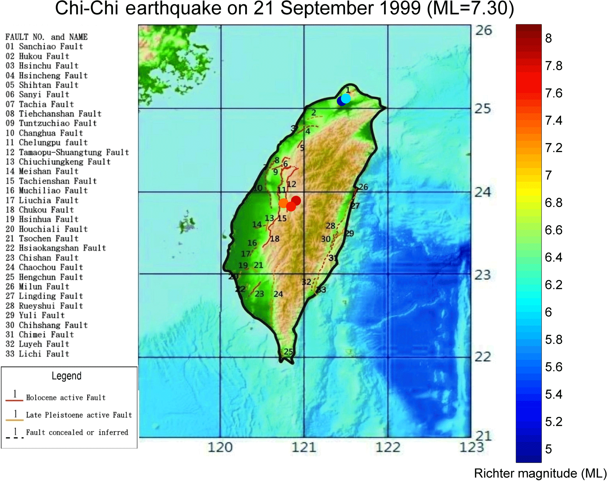
Figure 1The figure shows the position of Chelungpu fault (No. 11) on a map of Taiwan. Slip on this fault caused the Chi-Chi earthquake, which occurred at 01:47:15 on 21 September 1999 (TST), at a depth of 8.00 km, with a Richter magnitude (ML) of 7.3. The epicentre was at the coordinates (23.85∘ N, 120.82∘ E; Orange-coloured spot near the Chelungpu fault for No. 11). The four corresponding positions of the research stations are shown by a dark blue coloured spot (Station-TAP003), baby blue coloured (Station-TAP005) spot, red coloured spot (Station-TCU084) and dark red coloured spot (Station-TCU078) in this figure. Station-TCU078 is very close to the epicentre.
Lin (2017) performed the BPNN to predict the Physionet EMG signals. In that study, a modified M-LMA served as the backpropagation correction when training the BPNN. In this section, a newer modified M-LMA, called a modified elementary M-LMA, is introduced with the concept of an area element (surface element) to extend the simulation, e.g. for some surface problems instead of using line element in LMA, which is a function of an independent variable as stated previously. This algorithm is a modified version of the M-LMA used in Lin's study (2017). The algorithm can be transformed to a backpropagation correction in BPNN and is expected to have smaller predicted errors, following Lin's study (2017). In three-dimensional space, represented by three Cartesian coordinates (Descartes, 1667), a function of F is composed of two independent variables x and y. For simulated surface problems, the function F generates . The initial codomain is i=1; is defined as a target output (Rumelhart and McClelland, 1986). When xo and yo best satisfy the surface function to minimise εTε, the error is ; δxy can be defined as an area element when simulating a surface. Therefore, a Taylor-series expansion in two variations (δx and δy) approximates F as follows;
where Ja is defined as the Jacobian matrix with ; a series of (x1, y1), (x2, y2), and (x3, y3) is produced and converges toward a local minimiser , called an optimised output, so that can be estimated. When ε−Jaδxy is orthogonal to the column space of Ja and , I is defined as an identity matrix. A formula is proposed to import a parameter of r as follows:
Finally, Eq. (2) becomes
Here, is defined as the approximated Hessian matrix and rI=Ir, where r is the learning rate. In BPNN, if the learning rate is too high, the system will either oscillate about the true solution or it will diverge completely. If the learning rate is too low, the system will take a long time to converge on the final solution. In this study, based on the concepts in this section, the parameters x and y can serve as the weight and bias that can be simultaneously optimised with PDP in a BPNN (Fukushima, 1980) because of the concept of an area element, for a specially designated area element δxy used to simulate a optimised surface. Therefore when an x value is altered by a y value due to a specially designated relationship, real simultaneity can be achieved to simulate optimised area elements δxy (Abbena et al., 2006).
This means when an area element δxy is designated, then the x,y values related to δxy are simultaneously designated. Finally, an optimised surface is obtained from these elements. When simulating a surface with BPNN and LMA, which is a function of a variable (Lin, 2017), it serves as a backpropagation correction tool. A supposed initial x value is offered and is updated by a weight. The bias updates the y value. Both update processes are independent; without the concept of an area element, these processes are not simultaneous. In this situation, a simulated surface is obtained through simulating two nonlinear real-valued curves. One corresponds to the weight-updated x value, another corresponds to the y value, which has been updated by bias. Therefore, LMA is not a PDP for simulating a surface.
The results of many theoretical researches and engineering works regarding simulations have shown that using a two hidden layer network, with a small number of neurons in each layer, can replace a large number of neurons in a hidden layer network (Wagarachchi and Karunananda, 2014). The basic mathematical framework of an artificial neural network was already introduced in section 2 of the study by Lin (2017). Using the previously mentioned network framework, microseismic data, from the four stations stated in Sect. 1, serves as training data to build the new BPNN models after testing with different learning rates between 0 and 1, with an increment of 0.01, from which the magnitude of upcoming microseismic data will be predicted. The M-LMA introduced in Sect. 2 is used as the algorithm of backpropagation correction. For comparison, the LMA was simultaneously used as the algorithm of backpropagation correction. For both algorithm backpropagation, the initial weights and the initial biases were set to random variables (Nguyen and Widrow, 2009), and then feature scaling was performed (Bo et al., 2006; Xie et al., 2016). Using feature scaling, the variables were in the range of 0 and 1 because the value of the sigmoid function, called the activation function, which was used to train the BPNN in this study, was in the range of 0 to 1. Randomly distributing the weights between 0 and 1 helped prevent biases toward any particular output. If initialisation was non-random, the network would consistently and prematurely connect to certain outputs that were undermining the training. The 1000 epochs were given for sample signals in the seismic records (Sinha et al., 2010). The vertical component of an earthquake was the most dangerous because the earthquake forces mostly acted on the centre of gravity of the sliding soil mass, and the influences of vertical ground motions were on the seismic-induced displacements of the structures (Sawicki et al., 2007; Zhao et al., 2017). Therefore, these four vertical components, taken from the records, were predicted by the previously mentioned parameters and framework as a BPNN, using two hidden layers with 10 neurons in each layer to update the weight and bias to minimise backpropagation errors; these learning rates were found to be the best for minimising backpropagation errors. In this situation during training processing, the weights and biases would be updated, in which the neurons of BPNN were learning through updating the weights and biases as a PDP. The target output was defined as the size of the present signal at a last time point in the part of microseismic data of the records. The predicted error was defined as “target output subtracting expected output”. Therefore, the present time of the expected output, which was the predicted signal, was prior to the upcoming real signal. An expected output with a minimised predicted error was trended to build a BPNN model after training. Finally, when a BPNN model was used to predict the upcoming real signal, the designed instrument, including the hardware and software, were controlled to validate the present time of the predicted outputs between the two real seismic signals. Therefore, in this study, the computing speed of the designed instrument must be fast and stable to achieve this goal, which usually depended on the selected epoch in software (Sinha et al., 2010); for example, Matlab programme and hardware or computer conditions such as temperature of the CPU.
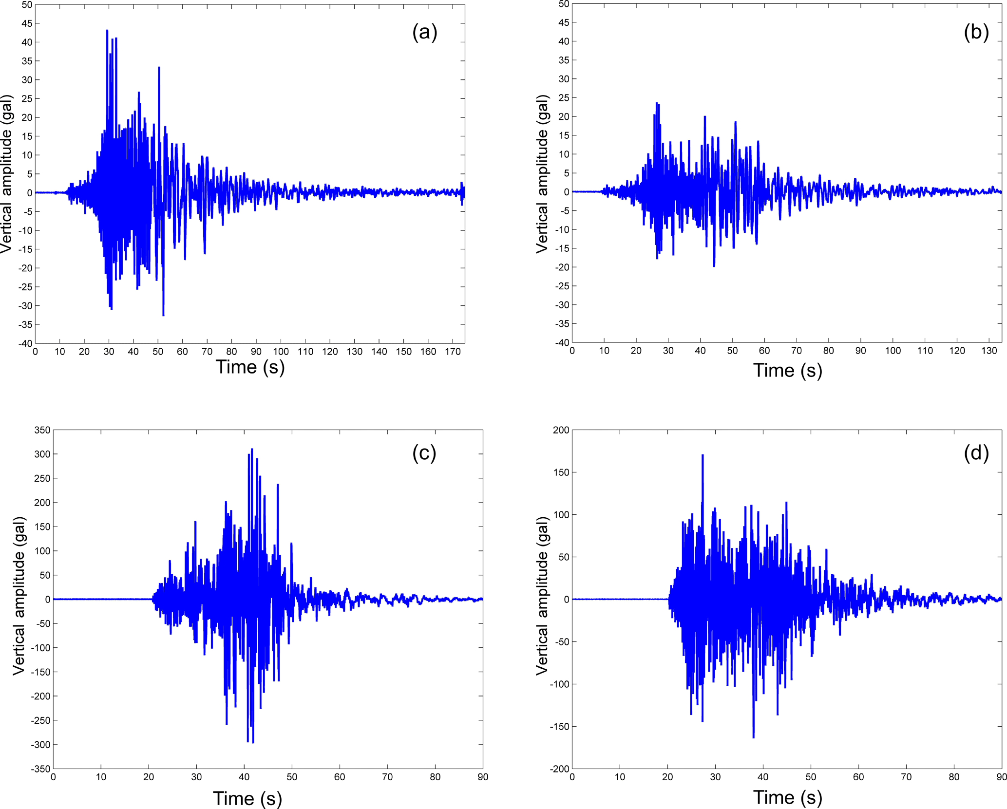
Figure 2(a) This figure shows the vertical component of the Chi-Chi earthquake. The unit of the record is gal (cm s−2. This was recorded by Station-TAP003 (25.08∘ N 121.45∘ E). (b) This figure shows the vertical component at Station-TAP005 (25.11∘ N 121.50∘ E) related to the Chi-Chi earthquake. (c) This figure shows the vertical component at Station-TCU084 (23.88∘ N 120.90∘ E) related to the Chi-Chi earthquake. (d) This figure shows the vertical component at Station-TCU078 (23.81∘ N 120.84∘ E) related to the Chi-Chi earthquake.
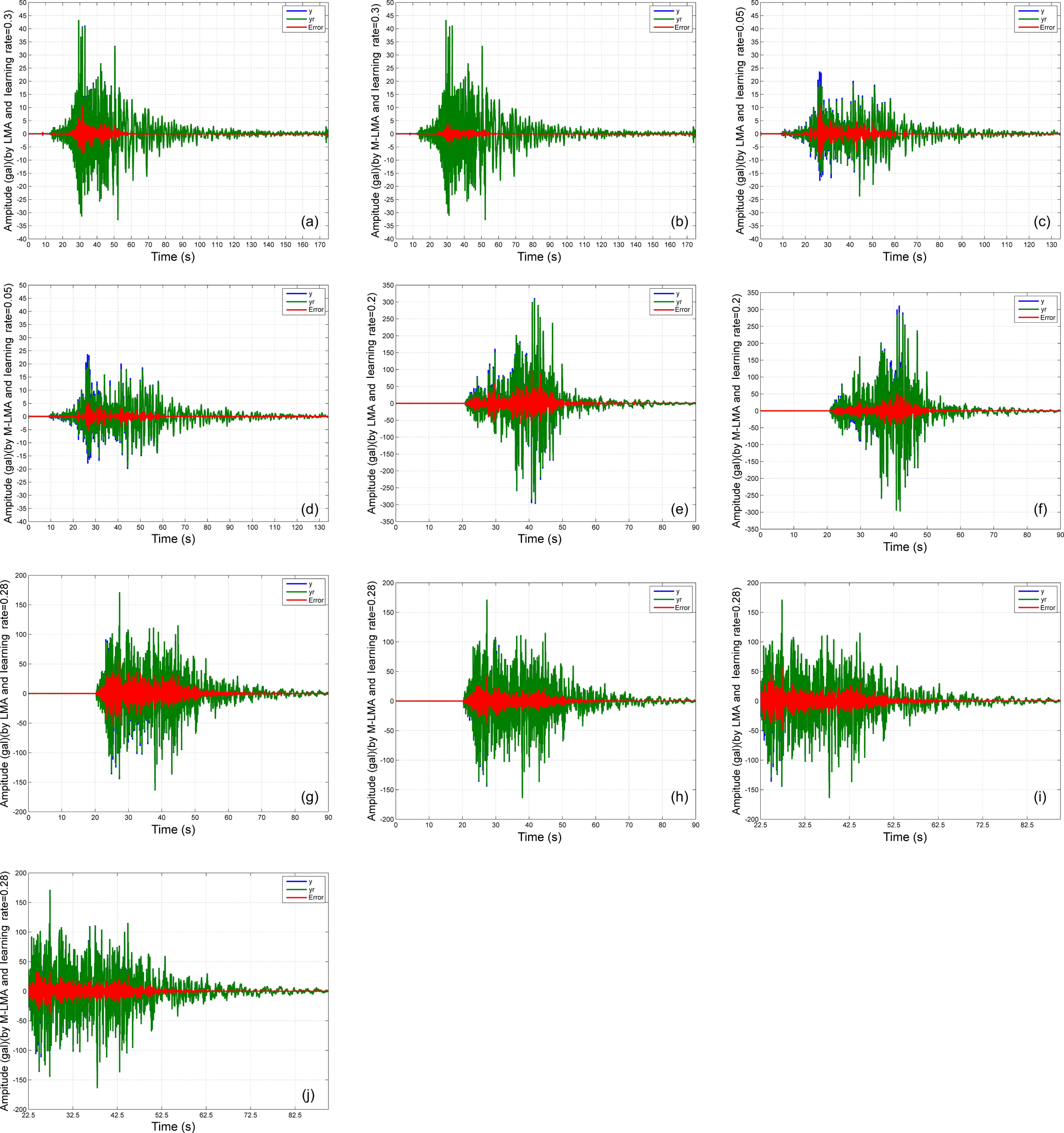
Figure 3(a) These two figures show the predicted results of the LMA and M-LMA of the signals shown in Fig. 2a, with a learning rate of 0.3. The predicted errors of the M-LMA are smaller than the LMA. The blue lines indicate the signals in Fig. 2a. The units are gal (cm s−2). The green lines indicate the outputs of the BPNN. The red lines indicate the predicted errors. (b) These two figures show the predicted results of the LMA and M-LMA of the signals shown in Figure 2b with a learning rate of 0.05. The predicted errors of the M-LMA are smaller. The blue lines indicate the signals in Fig. 2b. The green lines indicate the outputs of the BPNN. The red lines indicate the predicted errors. (c) The predicted results of the LMA and M-LMA of the signals shown in Fig. 2c using the same learning rate of 0.2. The predicted errors of the M-LMA are smaller. The blue lines indicate the signals in Fig. 2c. The green lines indicate the outputs of BPNN. The red lines indicate the predicted errors. (d) Predicted results of LMA and M-LMA for the signals shown in Fig. 2d, with a learning rate of 0.28. The predicted errors of the M-LMA are smaller. The blue lines indicate the signals in Fig. 2d. The green lines indicate the outputs of the BPNN. The red lines indicate the predicted errors. (e) These two figures show the predicted results of the LMA and M-LMA for the signals shown in Fig. 2d, with a learning rate of 0.28. However, the records are predicted at 22.5 s, after the beginning of strong motions due to the Chi-Chi earthquake. The predicted errors of the M-LMA are still smaller. The blue lines indicate the signals in Fig. 2d. The green lines indicate the outputs of the BPNN. The red lines indicate the predicted errors.
Figure 3a shows the predicted results of LMA and M-LMA with the same learning rate of 0.3 for records from Station-TAP003. The predicted results of M-LMA were better, with smaller predicted errors, compared to the results of LMA. Simultaneously, M-LMA was also shown to have better training with the microseismic data in the BPNN in order to produce a better BPNN model, and its processing was more similar to a biological neuron network with the PDP. Usually when the predicted errors were too large, then the predicting was lost, resulting in incorrect predicted upcoming data. Therefore, the results of the M-LMA were more meaningful and a significance was given for the predicting, when any anomalous output occurred, e.g. sudden amplified output with larger predicted error at approximately 9.5 s, prior to the strong motion at about 15 s, with a warning time of 5.5 s. It should be a good idea to use larger predicted errors as the predictors prior to the strong motion. Figure 3b presented the predicted results of the LMA and M-LMA, based on the records from Station-TAP005 using the best learning rate of 0.05 for both methods. The predicted results of the M-LMA were superior to those of the LMA, with smaller predicted errors. A sudden amplification in the output with large predicted errors occurred at approximately 9 s, which was nearly simultaneous with the start of strong motion and the first strong motion alert. Supposedly, the larger predicted error amplitudes, beginning from about 22 s, were seriously dangerous and a second strong motion alarm was sent, with a warning time of 13 s. Therefore, when predicting a record, the results of predicting must be similar to the larger amplitudes of predicted errors to avoid an erroneous secondary alarm. With this concept, a decision-making process using a suitable threshold of predicted error magnitudes at each station of the existing seismic monitoring network was necessary as second alarms from different stations. A decision-making process called “trade-off decision-making process with BPNN (TDPB)” was performed. In this study, the past records of the Chi-Chi earthquake were examined by TDPB, and then the thresholds were subjectively determined.
Different stations had different thresholds, and the selections of their suitable thresholds for secondary alarms should be calculated after being subject to significant testing in tandem with many stations in the same existing seismic monitoring network, and after observing the behaviours of waveforms for these records according to the many past earthquakes, including related microseismic methods. These suggested methods included nonlinear dynamic aseismic diagnosis (Xu et al., 2015; Ouazzani et al., 2017), surveying of the consideration of local building damages from past events under different local geological conditions that were evaluated by the earthquake-resistant and seismic coefficients, and seismic capacity evaluation of existing reinforced-concrete buildings (Moustafa, 2015).
Figure 3c presented the predicted results of the LMA and M-LMA from the proximal Station-TCU084 using the best learning rate for both methods, determined to be 0.2. The predicted results of the M-LMA had smaller predicted errors. A sudden amplification in the output, with large predicted error, occurred at approximately 22 s, which was almost simultaneous with the start of strong ground motion. The larger amplitudes beginning at about 34 s could be seriously dangerous and the warning time was 12 s. Figure 3d presents the predicted results of the LMA and M-LMA from near the Station-TCU078 using a best learning rate of 0.28 for both methods. The predicted results of the M-LMA, similar to the other stations, also had smaller predicted errors. A sudden amplification in the output, with large predicted error, occurred at approximately 21 s, which coincided with the start of strong motion. When large amplitudes beginning at around 27 s met real serious damages, and the warning time became 6 s. The TDPB was applied to avoid sending a false strong ground motion alarm, similarly to the aim previously stated about the decision-making process (Rath et al., 2017). For example, from the record of Station-TAP005 in Fig. 3b, a smaller predicted error occurred at about 9 s with the first alarm of strong motion, and through adjusting the threshold of the magnitude of the predicted errors, an alarm was sent at about 22 s, as previously stated, with a second alarm of strong motion in order to have a warning time of 13 s. When a sudden predicted error was first presented at a time point, and no sudden predicted error appears later, it would become misinformation, resulting in being defined as a “false alarm (nuisance alarm)” (Rath et al., 2017). The TDPB was suitable to solve this problem with a second alarm, similar to the processing of Iervolino et al. (2007). Therefore, for this topic, future research is necessary. If the seismic records record strong ground motion at 22.5 s, without a microseismic data, larger predicted errors would be found. Therefore, for this case, the microseismic data were necessary to train a BPNN model; the EEW was not validated without training microseismic data because the sudden predicted error appeared and it had no warning time. Figure 3e shows the predicted results of the LMA and M-LMA on the signals of Station-TCU084 with the same learning rate of 0.28. As previously stated, the processing of the method in this study was supplemented. The 1000 epochs were selected for Matlab 2013a in Windows 10 as the software, the computer hardware and seismic records with the same sampling rate of 200 Hz.
This BPNN approach was well suited, and it was unnecessary to consider the problems of characterising the wave phases and pre-processing, as stated previously. Furthermore, BPNN is a mature technology, which is expected to develop rapidly in the future, and does not require complex hardware. Determining an initial location and magnitude of the event is unnecessary for this technique. An existing seismic monitoring network, for example, the Free Field Strong Earthquake Observation Network of the CWB was already sufficient for these purposes. At each station in the monitoring network, adjusting the different leaning rates can minimise the predicted error. Therefore, all of the training records in the monitoring network would cause different station to have different learning rates. Finally, these BPNN models were built using the past microseismic data for sending second alarms through a decision-making process that belonged to post-mortem predicting. Therefore the warning time was retrieved afterwards. As stated previously, future research is necessary to apply real-time microseismic data to build the corresponding BPNN models. Such a nonlinear dynamic aseismic diagnosis may lead to TDPB so that warning time may be subjectively determined as soon as possible. However, this study has proposed this possibility for the EEW system which is different from previous works in Sect. 1 with the results of four stations.
M-LMA was determined to be better for predicting the vertical component of the Chi-Chi earthquake, using a learning rate of 0.3 for Station-TAP003. An anomalous output with larger predicted error was detected at about 15 s, and a sudden amplified output with smaller predicted error occurred at approximately 9.5 s prior to the strong motion due to the Chi-Chi earthquake. The warning time was 5.5 s. However, from the predicted results of the M-LMA with a learning rate of 0.05 related to Station-TAP005, a sudden amplified output was detected with large predicted error. This occurred at approximately 9 s, almost simultaneously with the initiation of strong motion. In this situation, using the TDPB , the large amplitudes starting at about 22 s had a warning time of 13 s. For Station-TCU084, which used a learning rate of 0.2, a sudden amplified output, with large predicted error, occurred at approximately 22 s, almost simultaneously with the starting of strong motion. When the TDPB was applied to larger amplitudes at about 34 s, the warning time became 12 s. For Station-TCU078, with a learning rate of 0.28, a sudden amplified output with large predicted error occurred at approximately 21 s. This coincided with the start of strong ground motion. When the TDPB was applied with larger amplitudes at about 27 s, and the warning time became 6 s. For these four recording stations, the M-LMA has been shown to produce smaller predicted errors. When predicting the records for these four stations, the sudden predicted errors, just after the microseismic data, could be considered as the beginning of the strong motion. Therefore, this method could serve as a real-time and online EEW tool, using an existing seismic monitoring network to assess the occurring risk of strong motions caused by a large earthquake, and considering the problems of characterising the wave phases and pre-processing was unnecessary. Complex hardware was also not required for the set-up.
The data are from the web site http://gdms.cwb.gov.tw/index.php, which requires an account and password. The data are available for research about earthquakes in the Southern Taiwan University of Science in Taiwan.
All authors have contributed to the research in this paper.
The authors declare that they have no conflict of interest.
The authors are grateful for the support of the Central
Weather Bureau, Taiwan, (CWB) for the data and the Ministry of Science and
Technology, Taiwan, under grant MOST 106-2221-E-218 -001 -MY2. This paper is especially in
memory of the death of the mother of the first author, “Lo, Yu-Mei” (8 November
1943–9 October 2016).
Edited by: Lev Eppelbaum
Reviewed by: two anonymous referees
Abbena, E., Salamon, S., and Gray, A.: Modern Differential Geometry of Curves and Surfaces with Mathematica, Textbooks in Mathematics, 3rd Edn., 1016 pp., Chapman and Hall/CRC, 2006.
Allen, R. M. and Kanamori, H.: The Potential for Earthquake Early Warning in Southern California”, Science, 300, 786–789, https://doi.org/10.1126/science.1080912, 2003.
Arjun, C. R. and Kumar, A.: Artificial neural network-based estimation of peak ground acceleration, ISET Journal of Earthq. Tech., Paper No. 501, 46, 19–28, 2009.
Bo, L., Wang, L., and Jiao, L.: Feature Scaling for Kernel Fisher Discriminant Analysis Using Leave-One-Out Cross Validation, Neural Computation, 18, 961–978, https://doi.org/10.1162/neco.2006.18.4.961, 2006.
Böse, M., Wenzel, F., and Erdik, M.: PreSEIS: A Neural Network-Based Approach to Earthquake Early Warning for Finite Faults, B. Seismol. Soc. Am., 98, 366–382, https://doi.org/10.1785/0120070002, 2008.
Brown, S. J., Caesar, J., and Ferro, C. A. T.: Global changes in extreme daily temperature since 1950, J. Geophys. Res., 113, D05115, https://doi.org/10.1029/2006JD008091, 2008.
Chen, L.: A modified Levenberg–Marquardt method with line search for nonlinear equations, Comput. Optim. Appl., 65, 753–779, 2016.
Descartes, R.: Discours de la methode: pour bien conduire sa raison, & chercher la verité dans les sciences: Plus La dioptrique, et Les meteores. Qui sont des essais de cette methode, A Paris: Chez Theodore Girard Salle du Palais, 414 pp., 1667.
Eslamian, S.: Handbook of Engineering Hydrology: Modeling, Climate Change, and Variability, Handbook of Engineering Hydrology, Vol.2, CRC Press, 646 pp., 2014.
Ferrier, D.: The Functions of the Brain”, London, Smith, Elder and Company, 1876.
Finsterle, S. and Kowalsky, M. B.: A truncated Levenberg–Marquardt algorithm for the calibration of highly parameterized nonlinear models, Comput. Geosci., 37, 731–738, https://doi.org/10.1016/j.cageo.2010.11.005, 2010.
Fukushima, K.: Neocognitron: A self-organizing neural network model for a mechanism of pattern recognition unaffected by shift in position, Biol. Cybern., 36, 93–202, https://doi.org/10.1007/BF00344251, 1980.
Gentili, S. and Michelini, A.: Automatic picking of P and S phases using a neural tree, J. Seismol., 10, 39–63, https://doi.org/10.1007/s10950-006-2296-6, 2006.
Iervolino, I., Giorgio, M., and Manfredi, G.: Expected loss-based alarm threshold set for earthquake early warning systems, Earthq. Eng. Struct. D., 36, 1151–1168, https://doi.org/10.1002/eqe.675, 2007.
Kecman, V.: Learning and soft computing: support vector machines, neural networks, and fuzzy logic models. Massachusetts Institute of Technology press, Cambridge, MA, 608 pp., 2001.
Kuyuk, H. S., Allen, R. M., H., Brown, M. H., Henson, I., and Neuhauser, D.: Designing a Network-Based Earthquake Early Warning Algorithm for California: ElarmS-2, B. Seismol. Soc. Am., 104, 162–173, https://doi.org/10.1785/0120130146, 2014.
Levenberg, K.: A method for the solution of certain non-linear problems in least squares, Q. Appl. Math., 2, 164–168, https://doi.org/10.1090/qam/10666, 1944.
Lin, J. W.: Backpropagation neural network (BPNN) as tracing method to trace physionet EMG signals: a case study, Advanced Studies in Medical Sciences, 5, 63–69, 2017.
Moustafa, A.: Earthquake Engineering – From Engineering Seismology to Optimal Seismic Design of Engineering Structures, InTech, 408 pp., https://doi.org/10.5772/58499, 2015.
Naveen, M., Jayaraman, S., Ramanath, V., and Chaudhuri, S.: Modified Levenberg Marquardt Algorithm for Inverse Problems, Asia-Pacific Conference on Simulated Evolution and Learning SEAL 2010: Simulated Evolution and Learning, 623–632, 2010.
Nguyen, D. and Widrow, B.: Improving the Learning Speed of 2-Layer Neural Networks by Choosing Initial Values of the Adaptive Weights, Information Systems Laboratory, Stanford University, Stanford, CA 94305, 2009.
Ouazzani, R. M., Salmon, S. J. A. J., Antoci, V., Bedding, T. R., Murphy, S. J., and Roxburgh, I. W.: A new asteroseismic diagnostic for internal rotation in Doradus stars, MNRAS, 465, 2294–2309, https://doi.org/10.1093/mnras/stw2717, 2017.
Pavlenko, V.: Ground motion variability and its effect on the probabilistic seismic hazard analysis, Thesis (PhD), The Faculty of Natural & Agricultural Sciences, University of Pretoria, Pretoria, 83 pp., 2017.
Peres, D. J. and Cancelliere, A.: Estimating return period of landslide triggering by Monte Carlo simulation, J. Hydrol., 541, 256–271, https://doi.org/10.1016/j.jhydrol.2016.03.036, 2016.
Rath, P. S., Barpanda, N. K., Singh R. P., and Panda, S.: A Prototype Multiview Approach for Reduction of False alarm Rate in Network Intrusion Detection System, IJCNCS, 5, 49–59, 2017.
Read, L. K. and Vogel, R. M.: Reliability, return periods, and risk under nonstationarity, Water Resour. Res., 51, 6381–6398, https://doi.org/10.1002/2015WR017089, 2015.
Rumelhart, D. E. and McClelland, J. L.: Parallel distributed processing, explorations in the microstructure of cognition, Vol. 1, 567 pp., Cambridge, MA, MIT Press, 1986.
Sawicki, A., Chybicki, W., and Kulczykowski, M.: Influence of vertical ground motion on seismic-induced displacements of gravity structures, Comput. Geotech., 34, 485–497, https://doi.org/10.1016/j.compgeo.2006.12.002, 2007.
Sinha, S., Singh, T. N., Singh, V. K., and Verma, A. K.: Epoch determination for neural network by self-organized map (SOM), Comput. Geosci., 14, 199–206, https://doi.org/10.1007/s10596-009-9143-0, 2010.
Shin, T. C., Tsai, Y. B., Yeh, Y. T., Liu, C. C., and Wu, Y. M.: International Handbook of Earthquake and Engineering Seismology, Vol 81B, 1057–1062, 2002.
Wagarachchi, N. M. and Karunananda, A. S.: Towards a Theoretical Basis For Modeling of Hidden Layer Architecture In Artificial Neural Networks”, Second International Conference on Advances in Computing, Electronics and Communication – ACEC 2014, Institute of Research Engineers and Doctors, USA, 47–52, https://doi.org/10.15224/978-1-63248-029-3-73, 2014.
Wu, S., Beck, J. L., and Heaton, T. H.: ePAD: Earthquake Probability-Based Automated Decision-Making Framework for Earthquake Early Warning, CACAIE, 28, 737–752, https://doi.org/10.1111/mice.12048, 2013.
Wu, Y. M. and Kanamori, H.: Development of an Earthquake Early Warning System Using Real-Time Strong Motion Signals, Sensors, 8, 1–9, https://doi.org/10.3390/s8010001, 2008.
Wu, Y. M. and Teng, T. I.: A Virtual Subnetwork Approach to Earthquake Early Warning, B. Seismol. Soc. Am., 92, 2008–2018, https://doi.org/10.1785/0120010217, 2002.
Xie, L., Tian Q., and Zhang, B.: Simple Techniques Make Sense: Feature Pooling and Normalization for Image Classification, IEEE T. Circ. Syst. Vid., 26, 1251–1264, https://doi.org/10.1109/TCSVT.2015.2461978, 2016.
Xu, Z., Ren, C., and Xiao, C.: The ASeismic Design and Nonlinear Dynamic Analysis of a 350 m High Braced Steel Frame, CTBUH 2015 New York Conference, 561–568, 2015.
Yazdani, A., Salehi, H., and Shahidzadeh, M. S.: A modified three-parameter lognormal distribution for seismic demand assessment considering collapse data, KSCE J. Civ. Eng., 22, 204–212, https://doi.org/10.1007/s12205-017-1820-2, 2018.
Zhao, L. H., Cheng, X., Dan, H. C., Tang, Z. P., and Zhang, Y.: Effect of the vertical earthquake component on permanent seismic displacement of soil slopes based on the nonlinear Mohr–Coulomb failure criterion, Soils Found., 57, 237–251, https://doi.org/10.1016/j.sandf.2016.12.002, 2017.