the Creative Commons Attribution 4.0 License.
the Creative Commons Attribution 4.0 License.
 | 24 Sep 2019
Evaluations of an ocean bottom electro-magnetometer and preliminary results offshore NE Taiwan
Ching-Ren Lin
Chih-Wen Chiang
Kuei-Yi Huang
Yu-Hung Hsiao
Po-Chi Chen
Hsu-Kuang Chang
Jia-Pu Jang
Kun-Hui Chang
Feng-Sheng Lin
Saulwood Lin
Ban-Yuan Kuo
The first stage of field experiments involving the design and construction of a low-power consumption ocean bottom electro-magnetometer (OBEM) has been completed, which can be deployed for more than 180 d on the seafloor with a time drift of less than 0.95 ppm. To improve the performance of the OBEM, we rigorously evaluated each of its units, e.g., the data loggers, acoustic parts, internal wirings, and magnetic and electric sensors, to eliminate unwanted events such as unrecovered or incomplete data. The first offshore deployment of the OBEM together with ocean bottom seismographs (OBSs) was performed in NE Taiwan, where the water depth is approximately 1400 m. The total intensity of the magnetic field (TMF) measured by the OBEM varied in the range of 44 100–44 150 nT, which corresponded to the proton magnetometer measurements. The daily variations in the magnetic field were recorded using the two horizontal components of the OBEM magnetic sensor. We found that the inclinations and magnetic data of the OBEM varied with two observed earthquakes when compared to the OBS data. The potential fields of the OBEM were slightly, but not obviously, affected by the earthquakes.
- Article
(7899 KB) - Full-text XML
- BibTeX
- EndNote


Marine electromagnetic exploration is a geophysical prospecting technique used to reveal the electrical resistivity features of the oceanic upper mantle down to depths of several hundreds of kilometers in different geologic and tectonic environments, such as in areas around mid-oceanic ridges, areas around hot-spot volcanoes, subduction zones, and normal ocean areas between mid-oceanic ridges and subduction zones (Ellis et al., 2008; Evans et al., 2005; Key, 2012; Utada, 2015).
Table 1Specifications of the OBEM compared to the Japanese OBEM and OBE (Kasaya and Goto, 2009).
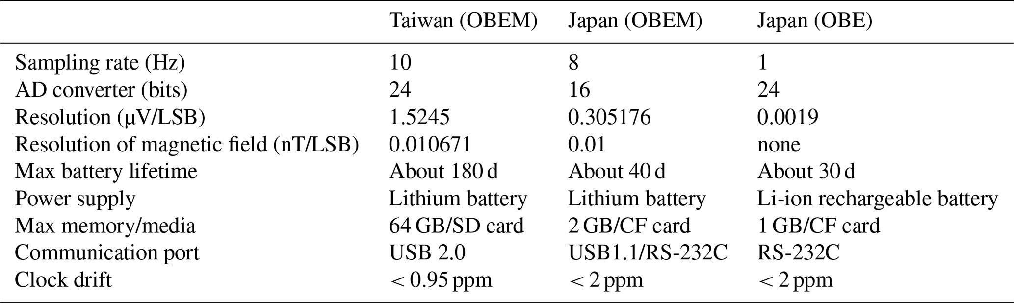
Even though many magnetotelluric explorations have investigated deep electrical structures on Taiwan (Bertrand et al., 2009, 2012; Chiang et al., 2011, 2010, 2015, 2008), there were no marine electromagnetic experiments around Taiwan until 2010. The first generation of ocean bottom seismographs (OBSs) was developed by the Institute of Earth Sciences, Academia Sinica (IES), Taiwan Ocean Institute, National Applied Research Laboratories, and the Institute of Undersea Technology, National Sun Yat-sen University (OBS R&D team), in 2009, called Yardbird-20s. These OBSs have acquired large amounts of data via a series of deployments offshore Taiwan that can be used to study plate tectonics and crustal characteristics (Kuo et al., 2015, 2012, 2014). Subsequently, the OBS R&D team developed an ocean bottom electro-magnetometer (OBEM) modified from the OBS based on important developmental experiments.
The novel OBEM was constructed by the OBS R&D team and has completed the first stage of field experiments by the Institute of Earth Sciences, National Ocean Taiwan University, and IES. One OBEM and six broadband OBSs, called Yardbird-BBs (Broadband Yardbirds), were deployed at the western end of the Okinawa Trough (OT), NE Taiwan, for field testing in March 2018. The water depth in this area is approximately 1400 m. All the instruments were successfully recovered in May 2018 after collecting the first OBEM field data in Taiwan. Here, we introduce the OBEM design, specifications, calibration procedures, and its further developments and improvements.
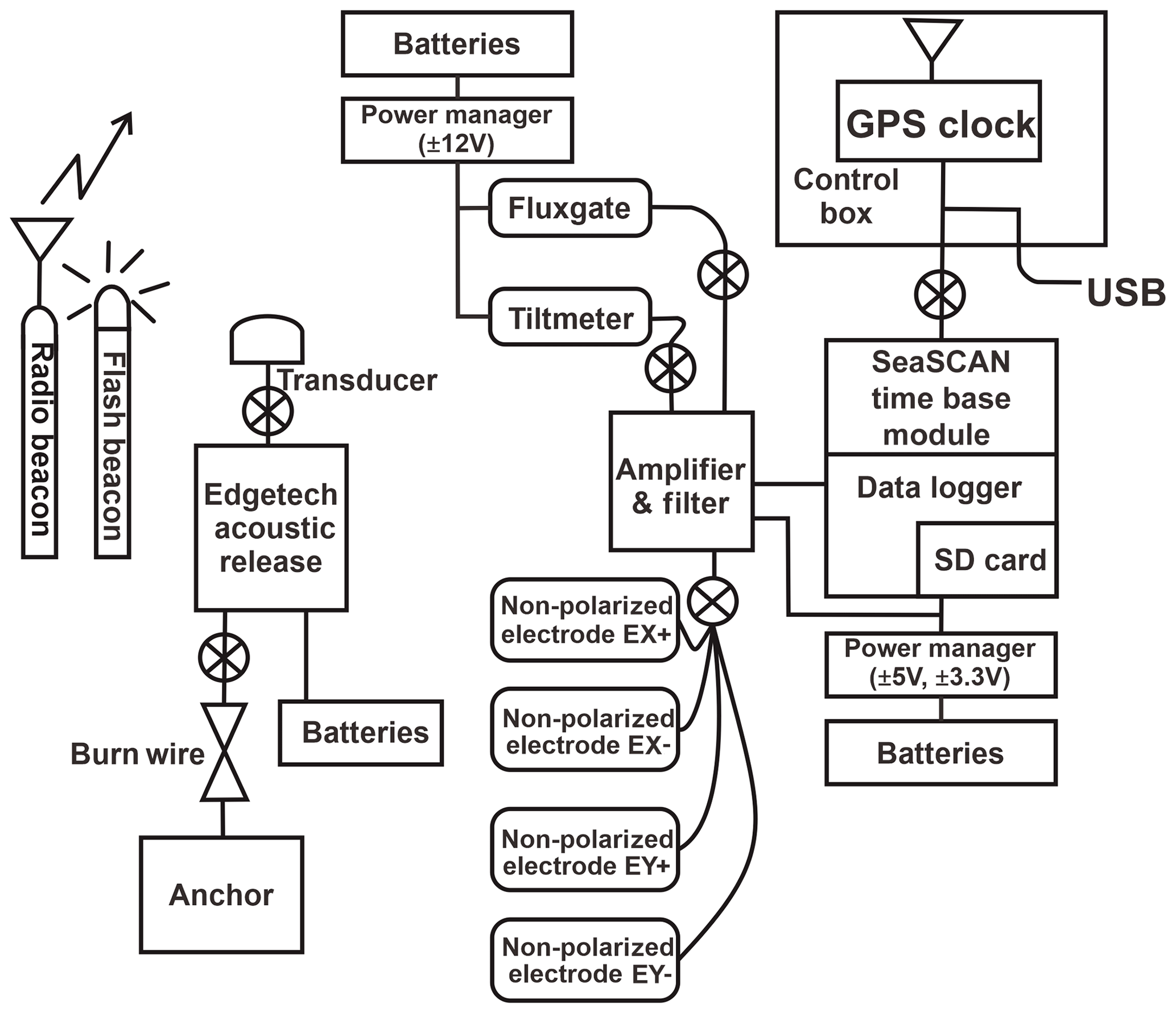
Figure 1A block diagram of the OBEM. The inputs of the two electric fields, two inclinations and three magnetic fields pass through the Amp & LPF in the data logger, which contains a 64 GB SD card. The SeaSCAN time base module is integrated into the data logger and has a timing error smaller than 3 s yr−1. The EdgeTech acoustic transceiver and transducer are used for the positioning and releasing of the anchor. The radio and flash beacons are used to locate the OBEM at the sea surface during recovery operations.
The OBEM is designed to be wireless deep underwater equipment; however, the power supply is limited for the wireless OBEM because the batteries cannot be directly charged via electric cables from vessels. Therefore, designing low-power consumption for the OBEM and high-efficiency battery packs is critically required for long periods of operation. The major units of the OBEM include a data logger, a magnetic sensor, a tiltmeter, electric receivers with an arm-folding mechanism, a relocation system, recovery units and an anchor. All the units for the OBEM use nonmagnetic materials (e.g., the screws and anchor). Figure 1 shows a block diagram of the OBEM, whereas the specifications of the OBEM compared to the Japanese system (Kasaya and Goto, 2009) are shown in Table 1. We designed the data logger, release mechanism and the OBEM platform to integrate all the sensors or units purchased from related manufacturers and focused on the issues of saving power and reducing costs. The detailed requirements of the OBEM are listed below.
-
A magnetic sensor with three axes for measuring magnetic fields.
-
A tiltmeter with two axes for measuring leveling changes to correct the tilt error of the magnetic sensor.
-
Two pairs of non-polarized electrodes with 2 m bendable arms with a total distance between the electrodes of approximately 4.5 m.
-
A highly accurate data logger with at least seven channels and a sampling rate of greater than or equal to 10 samples per second (SPS).
-
Operation time of more than 180 d.
-
An internal timing error of less than 3 s yr−1 synchronized with GPS.
-
Acoustic relocation and recovery control systems.
-
Power consumption of less than 1.5 W.
-
A radio beacon, flush beacon, reflect label and orange flag for identification on the sea surface during instrument recovery.
-
A 0.75 m s−1 subside rate for deployment and float-up rate for recovery.
-
A maximum deployment depth of more than 6000 m appropriate for most seawater depths offshore Taiwan.
The solutions found for the OBEMs are listed below.
-
A fluxgate with three axes with a sensitivity of ±70 000 nT and a noise level < 6 pTrms/√Hz at 1 Hz adding a buffer amplifier with gain = 0.2 and passive low-pass filter at 50 Hz; the scaling temperature coefficient is ±15 ppm ∘C−1, whereas the offset temperature coefficient is ±0.1 nT ∘ C−1.
-
Four non-polarized electrodes (Ag ∕ AgCl), with a self-noise level < 625 µV adding a buffer amplifier with gain = 20 and two active low-pass filters at 50 Hz.
-
A tiltmeter with two axes with inclinations of ±30∘ adding a buffer amplifier gain = 0.2 and a passive low-pass filter at 50 Hz.
-
Two pairs of silver chloride electrodes with a 2 m arm-folding mechanism.
-
A low-noise and low-power consumption eight-differential channel 24 bit A/D data logger with an accurate internal timing clock.
-
Acoustic transponder and controller units.
-
Radio beacon and flash beacon units.
-
An OBEM platform modified from that of OBS.
-
High-efficiency lithium battery packs for the sensors and data logger.
The OBEM is recovered by releasing its anchor from the seafloor via an onboard acoustic command. The OBEM is returned to the sea surface via buoyancy when the anchor is released. There are two typical release mechanisms available for OBEMs to unlock their anchors: spin motor and burn-wire systems (Kasaya and Goto, 2009). The OBEM uses the burn-wire system because it weighs less than the spin motor system. The acoustic controller and transducer use ORE #B980175 ASSY PCB and #D980709, respectively, manufactured by EdgeTech, USA, for the corresponding functions of OBEM recovery and underwater ranging. The ASSY PCB acoustic controller uses a binary FSK (frequency-shift keying) encoder, including the commands “RELEASE1”, “RELEASE2”, “DISABLE”, “ENABLE” and “OPTIONAL1”. The frequency of the acoustic range ranges from 7.5 to 15 kHz in increments of 0.5 kHz with a sensitivity of 80 dB re 1 V muPa−1. The #D980709 transducer can work at a depth of 6000 m and in environments from −10 to +40 ∘C.
The EdgeTech 8011M model acoustic commander (8011M) is used on board to send the ENABLE command to open the ranging function, the “RANGE” command to measure the distance between the OBEM and the research vessel, the DISABLE command to close the ranging function, and the RELEASE1 command to activate the burn-wire system to release the anchor. The RELEASE1 command persists for 15 min unless terminated by the OPTIONAL1 command.
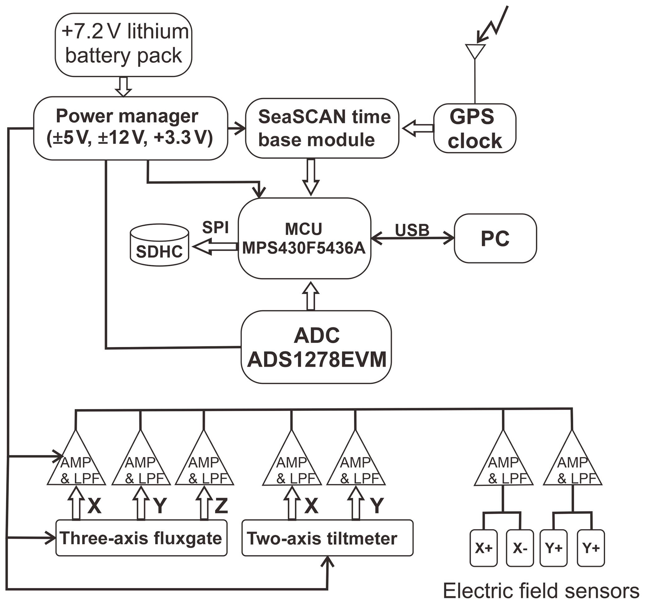
Figure 2A block diagram of the OBEM data logger. The ADS1278EVM is a 24 bit A/D with eight inputs used for converting analog signals via the amplifier and low-pass filter (Amp & LPF) to digital data. The Amp & LPF adjusts the output voltages of the sensors of the fluxgate, tiltmeter and electric receivers to suitable A/D input levels. The two MCUs of the MPS430F5436A process the timing synchronization by the SeaSCAN of time base and GPS modules, the digital data storage to the SD card with a standard SDHC, and the user interface communication with a PC.
We selected the RF-700A and ST-400A NOVATECH models for the radio and flash beacons, respectively, for use in the OBEM. The maximum deployment depth for these models is 7300 m. The radio beacon is turned ON by sending a VHF (very high-frequency) signal, and the flush beacon is turned ON at atmospheric pressure of less than 1 atm (equal to a depth of 10 m below the sea surface) in a dark environment. The beacons are also turned OFF at a depth of 10 m or at atmospheric pressure of less than 1 atm, respectively. These two beacons have four independently installed C-type alkaline batteries that allow for 6 d of continuous operation at a maximum; this power supply differs from that of the data logger. The two independent power supply layouts allow the beacons to properly operate even if the power supply for the data logger fails. An onboard radio scanner detects the signal transmitted from the radio beacon at a distance of 6.4–12.9 km when the OBEM is floating on the surface. These two beacons can assist in locating the OBEM on the sea surface in both daytime and nighttime.
TL-5930 model lithium batteries manufactured by TADIRAN are used for the OBEM, with specifications of 3.6 V, 19 Ah and a D type, with characteristics of high energy density and a low self-discharge rate suitable for long periods of operation. Figure 2 shows a block diagram of the OBEM data logger. The ADC1278EVM model is a 24 bit A/D converter used for the inputs of the three fluxgate axes, the two tiltmeter axes and two pairs of non-polarized electrodes with a sampling rate of 10 SPS. An amplifier and a low-pass filter (Amp & LPF) were designed for the magnetic sensor, leveling sensor and electric receiver inputs. The two MPS430F5436A microcontrollers (MCUs) process the timing synchronization of the time base manufactured by SeaSCAN, USA, and the GPS modules; the digital data are stored on a Secure Digital (SD) memory card with a standard Secure Digital High Capacity (SDHC), and the user interface communicates with a PC. The time base module supplies a precise time base signal to the data logger, whereas the SISMTB Ver 4.1 time base module generates a precise 125 Hz clock that supports a timing error smaller than 3 s yr−1. Even though the time base module supports a very small timing error of 3 s yr−1, the data logger clock is still synchronized with the GPS on deck for timing corrections after recovering the OBEM. The maximal capacity of the SD card is 64 GB and can support data storage for more than 1 year with a sampling rate of 10 SPS.
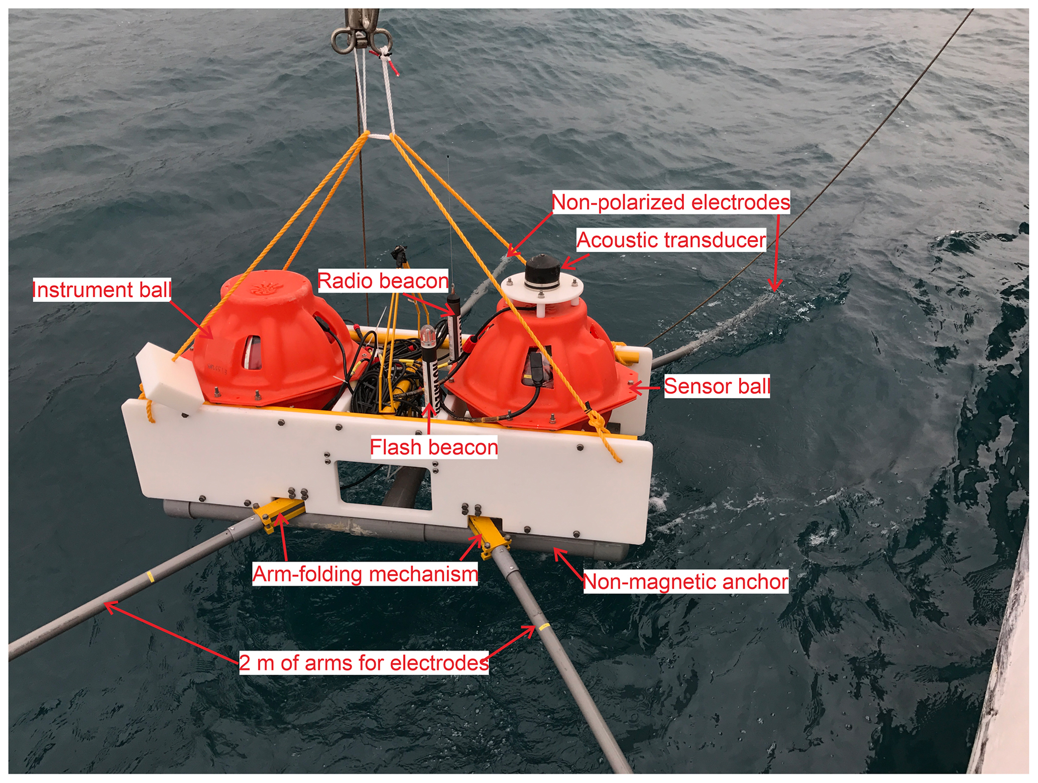
Two 17 in. glass VITROVEX spheres manufactured by Nautilus Marine Service GmbH, Germany, are used for the OBEM. These glass spheres contain the fluxgate and tiltmeter (sensor ball) and the seven channels of the Amp & LPF, data logger, #B980175 ASSY PCB acoustic controller and batteries (instrument ball) and can be deployed at a depth of 6000 m and support a total buoyancy of 52 kg. The instrument and sensor balls, the silver chloride electrodes, and the burn-wire system are connected via waterproof cables. There is a pressure-vacuum valve outside the glass spheres that allows a pumped vacuum to be preserved at 0.7 atm; self-fusing butyl rubber tape is used to fill the suture zone between the half glass spheres. In addition, two crossed stainless-steel bands are used to improve the waterproofing of the glass spheres and cover the orange PE cases. Four PVC pipes with lengths of 2 m are combined to form the OBEM platform for the electric receivers, and the silver chloride electrodes are installed at the ends of the pipes. A 60 kg nonmagnetic anchor is attached to the bottom of the OBEM platform and catches via a releasing mechanism. The anchor can be released using the burn-wire system to recover the OBEM. Figure 3 shows a photograph of the OBEM platform.
It is necessary to calibrate each unit of the OBEM, including the data logger with the Amp & LPF, fluxgate, tiltmeter, electrodes, ASSY PCB acoustic controller, transducer and wiring, before and after assembling the OBEM to improve its performance. We describe the series of calibration methods used for the OBEM units in the following section.
4.1 Calibrations of the background noise of the data logger and the Amp & LPF
The background noise of the data logger is defined as
where n is a data point and A1 to An indicate the amplitudes of the data points, 1 to n, individually at the short circuit or 0 V. The background noise of the data logger (in “BIT”) is calculated as
The data logger contains seven input channels called MX, MY, MZ, TX, TY, EX and EY. MX, MY and MZ are used for the magnetic sensor of the fluxgate, TX and TY are used for the tiltmeter, and EX and EY are used for the electric receivers. The calibration procedure is described below.
-
Connect MX, MY, MZ, TX and TY to GND (Ground), EX+ with EX− and EY+ with EY−.
-
Start the record mode of the data logger, wait for 60 s to acquire data, and then stop recording data.
-
Download the data from the data logger and convert it to ASCII format. Then, calculate the background noise using Eq. (1) and the background noise in dB using Eq. (2).
4.2 Calibrations of the sensitivity, linearity error and dynamic range for the data logger and the Amp & LPF
The input ranges of the voltages for MX, MY and MZ are ±10 V, for TX and TY they are ±5 V, and for EX and EY they are ±0.00625 V. The sensitivities are calculated from the average count of the input voltages; that is, subtract the average count at zero voltage and then divide by the input voltages:
where Vi is the input voltage, Ci is the output count saved on the SD card for an input voltage of Vi, and C0 is the output count saved on the SD card for an input voltage of 0 V. The linearity errors are calculated such that
where Si is the sensitivity of the input voltage and ST is the total sensitivity.
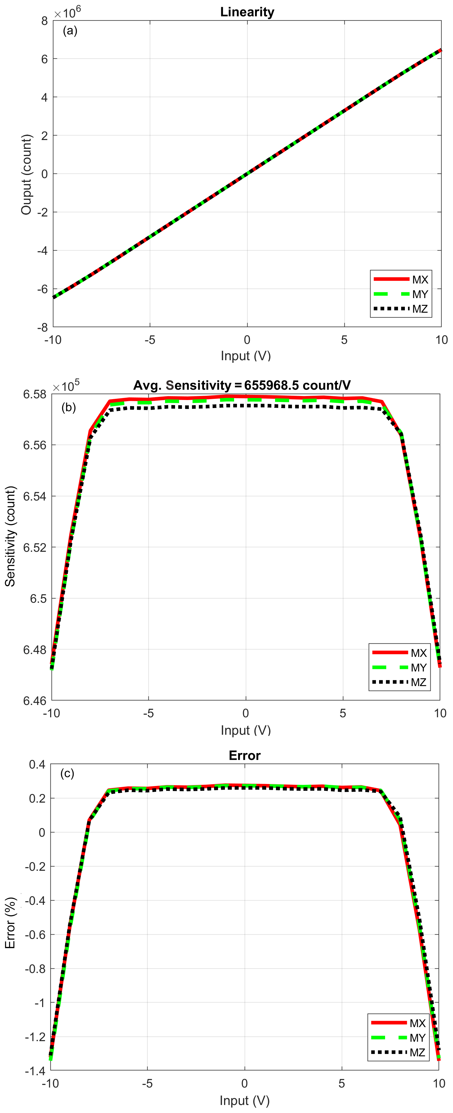
Figure 4Calibration results for the magnetic channels of the OBEM01. (a) Linearity, (b) sensitivity and (c) error. The average sensitivity is 655 968.5 counts V−1, and the maximum error is < 1.35 %.
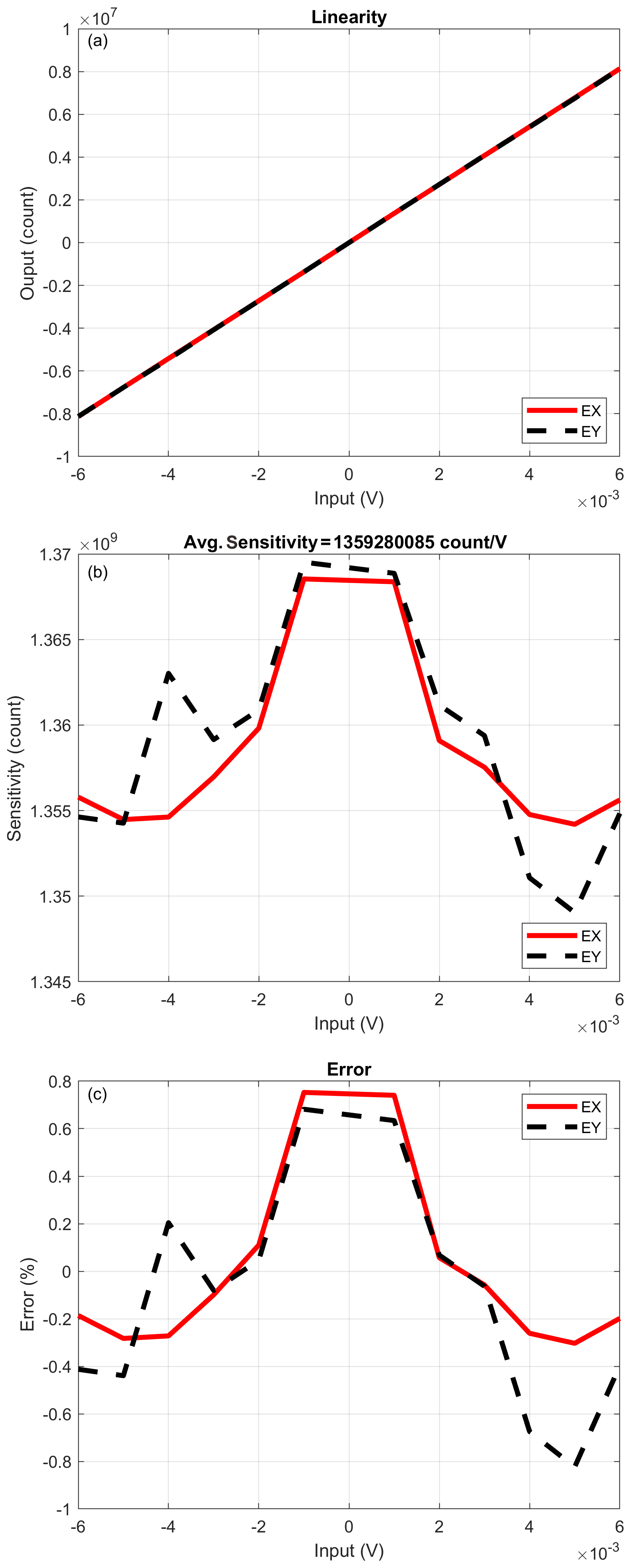
Figure 5Calibration results for the electric channels of the OBEM01. (a) Linearity, (b) sensitivity and (c) error. The average sensitivity is 1 358 568 047.8 counts V−1, and the maximum error is < 0.8 %.
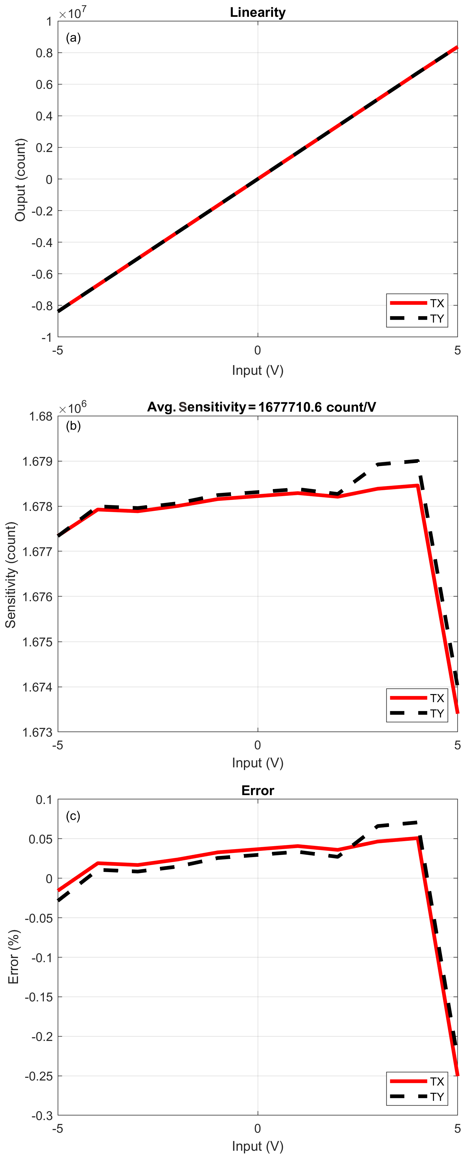
Figure 6Calibration results for the inclination channels of the OBEM01. (a) Linearity, (b) sensitivity and (c) error. The average sensitivity is 1 677 710.6 counts V−1, and the maximum error is < 0.25 %.
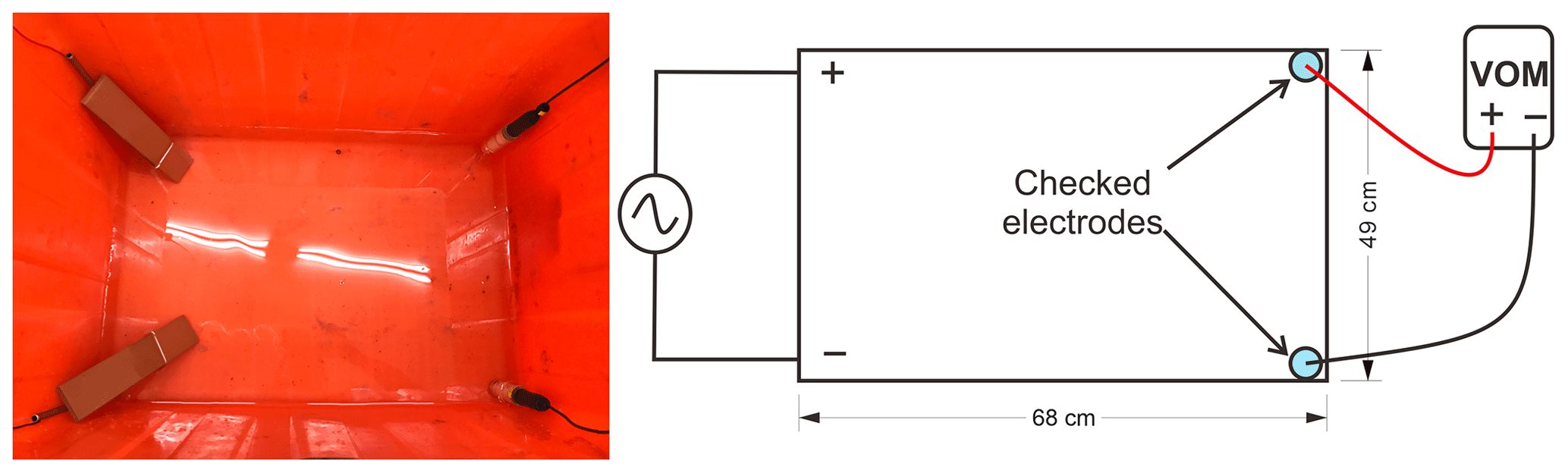
Figure 7The layout for the evaluation of the electric receivers. Two copper electrodes are used to vary the input signals. A pair of silver chloride electrodes are placed at the corner of a tank with an area of 68 cm × 49 cm filled with 15 cm of seawater. A VOM is used to measure the self-potential and impedance of the electrodes.
The dynamic range is the ratio of the maximum count to the background noise. It is defined as
where ST is the total sensitivity and Vmax is 10 V for MX, MY and MZ, 5 V for TX and TY, and 0.00625 V for EX and EY. Its calibration procedure is described below.
-
Connect the MX, MY and MZ channels of the data logger to the source voltages generated by the calibrator (FLUKE726) and connect the GND channel of the data logger to the source common point (COM) of FLUKE726.
-
Set the data logger to the recording mode.
-
Set the FLUKE726 output voltages from 0 to ±10 V. Increase and decrease the voltages step by step at 1 V intervals until ±10 V. The measurement time length for each output voltage is 20 s.
-
Connect the TX and TY channels of the data logger to the source voltages generated by FLUKE726 and connect the GND channel of the data logger to the COM of FLUKE726.
-
Set the FLUKE726 output voltages from 0 to ±5 V. Increase and decrease the voltages step by step at 1 V intervals until ±5 V. The measurement time length for each output voltage is 20 s.
-
Connect the EX+ and EY+ channels of the data logger to the source voltages generated by FLUKE726, and connect the EX− and EY− channels of the data logger to the COM of FLUKE726.
-
Set the FLUKE726 output voltages from 0 to ±6 mV. Increase and decrease the voltages step by step at 1 mV intervals until ±6 mV. The measurement time length for each output voltage is 20 s.
-
Finally, switch off the recording mode of the data logger, download the data and convert it to ASCII format for analysis. Calculate the sensitivity, linearity error and dynamic range using Eqs. (3), (4) and (5), respectively.
Figure 4 shows a calibration of the magnetic channels (MX, MY and MZ) checking the sensitivity, linearity and error. The average sensitivity is 655 968.5 counts V−1 with a maximum error smaller than 1.35 %. Figure 5 shows a calibration of the electric channels (EX and EY) checking the sensitivity, linearity and error. The average sensitivity is 135 856 047.8 counts V−1 with a maximum error smaller than 0.8 %. Figure 6 shows a calibration of the tiltmeter channels (TX and TY) checking the sensitivity, linearity and error. The average sensitivity is 1 677 710.6 counts V−1 with a maximum error smaller than 0.25 %. The noise level of the data logger is 57.8 dB, whereas its dynamic range is 80.2 dB at 10 Hz.
4.3 Evaluation of the current consumption
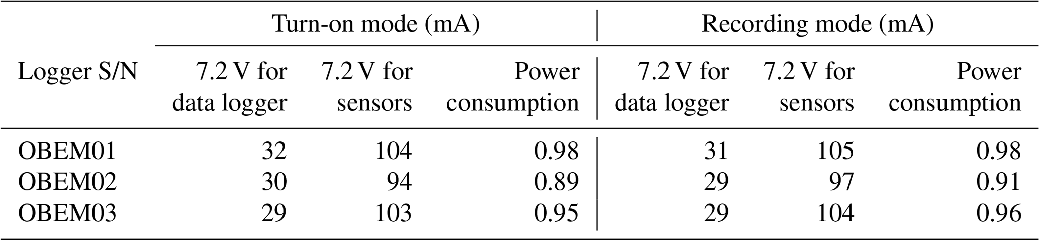
The power supplies of the OBEM consist of two 7.2 V battery packs in a series connection with two 3.6 V lithium batteries. One battery pack is for the data logger and converts to ±5 and +3.3 VDC (voltage direct current). The other pack is for the sensors and converts to ±5 and +12.0 VDC. Two +7.4 VDC output current batteries were measured for their current consumption measurement using two ammeters connecting the two +7.4 V battery packs. Table 2 shows the current consumption of the OBEM system. The maximum current consumptions of the data logger and sensors are 32 and 105 mA, respectively. The total power consumption is less than 1 W, which corresponds to expectations.
4.4 Evaluation of the electrodes
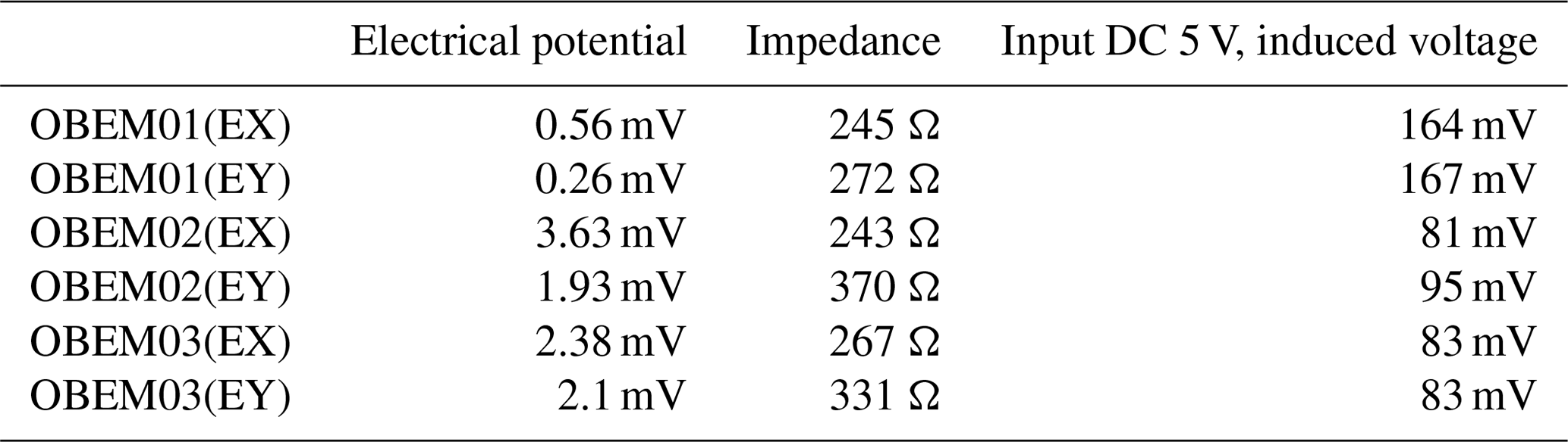
Two pairs of silver chloride electrodes are used for the OBEM. We first put a pair of electrodes separated by a fixed distance within a tank filled with seawater to check the status of the electrodes. Second, we measured the electrical potential and impedance of the electrodes using a digital volt–ohm–milliammeter (VOM) (Fig. 7). Third, we sent a swept sine signal to check the frequency responses of the electrodes, as shown in Fig. 8. Fourth, we input a DC voltage to check the electrode-induced voltages, as shown in Fig. 9. Table 3 shows the self-potential, impedance and induced voltages for each pair of electrodes. The ranges of the self-potential and impedance are 0.26–3.63 mV and 243–370 Ω, respectively. The electrical potential shows that 81–167 mV was transmitted from the 5 VDC of the two copper electrodes.
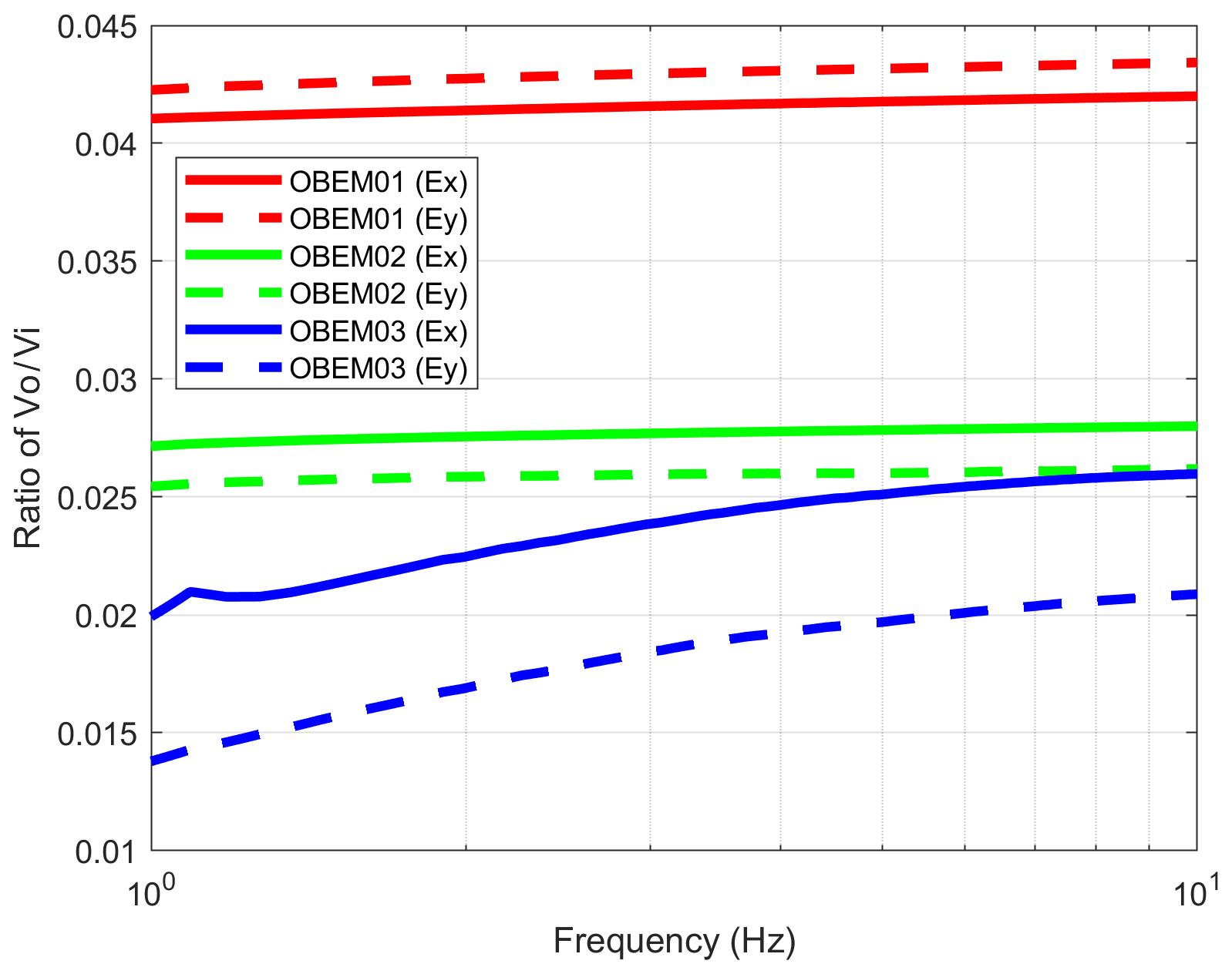
Figure 8The responses of the electrodes with varying frequencies. The response curves of Vo∕Vi are proportional to the frequency on a log scale.
Table 3The self-potential, impedance and induced voltage results for each pair of silver chloride electrodes.
4.5 Evaluation of the fluxgate
The fluxgate is mounted in the sensor ball of the OBEM. Therefore, we could only calculate the total magnetic field (TMF) (Eq. 6) measured from the three components of the fluxgate. We then compared the difference between the TMF of the OBEM and geomagnetic data of the geophysical database management system from the Central Weather Bureau. The TMF is calculated by
where MX, MY and MZ are the components of the north–south, east–west and vertical magnetic fields, respectively.
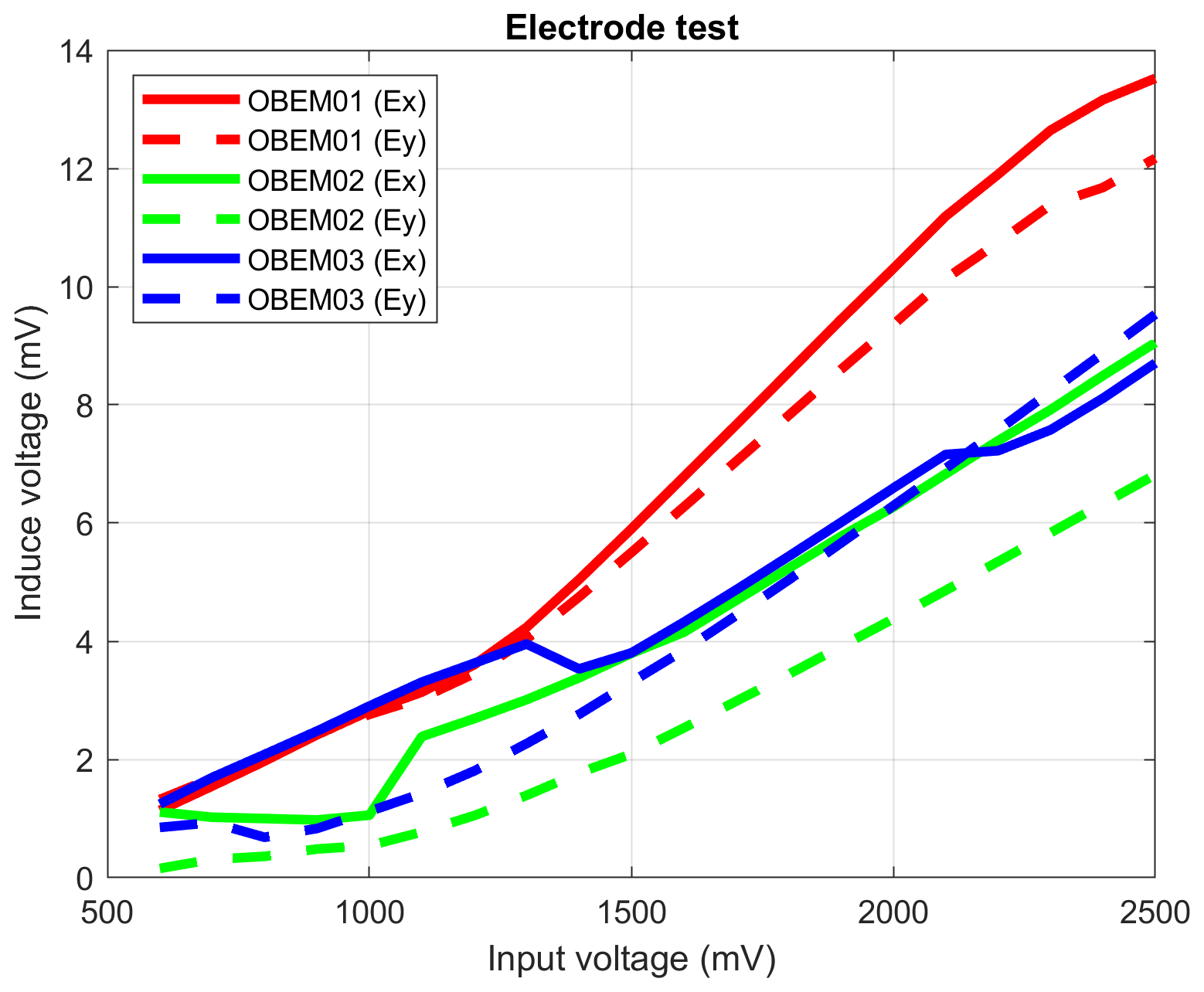
Figure 9The responses of the electrodes with varying voltages. The input ranged from 500 to 2500 mVDC to check the induced voltage; the induced voltages are proportional to the input voltages.
4.6 Evaluation of the acoustic transceiver and its transducer
We selected the large-scale Breeze Canal in New Taipei City for testing because it has few obstacles and is suitable for evaluating the functions of the 8011M. The Breeze Canal has a length of approximately 800 m and is located in a straight river with a depth of 2–5 m. The distance between the transducer and the acoustic transceiver was approximately 630 m, and the layout for the field test is shown in Fig. 10. The testing procedure for the transducers is described below. The results are listed in Table 4.
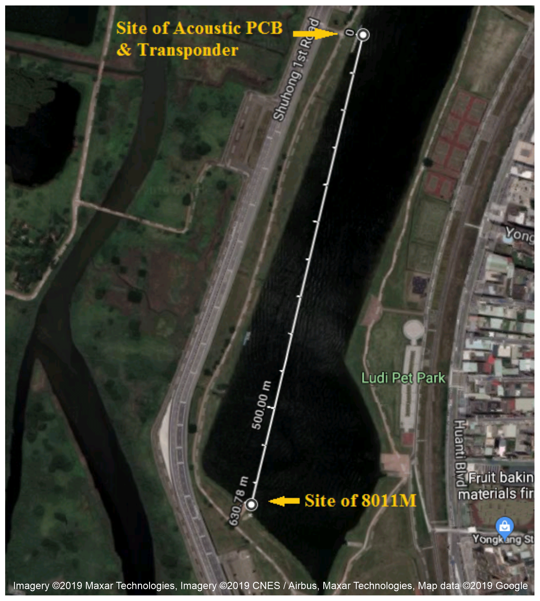
Figure 10A map of the field test to evaluate the acoustic transducer, acoustic controller and 8011M (modified from Google Maps, https://www.google.com.tw/maps/@25.0902745,121.4516598,1296m/data=!3m416, last access: 19 August 2019).
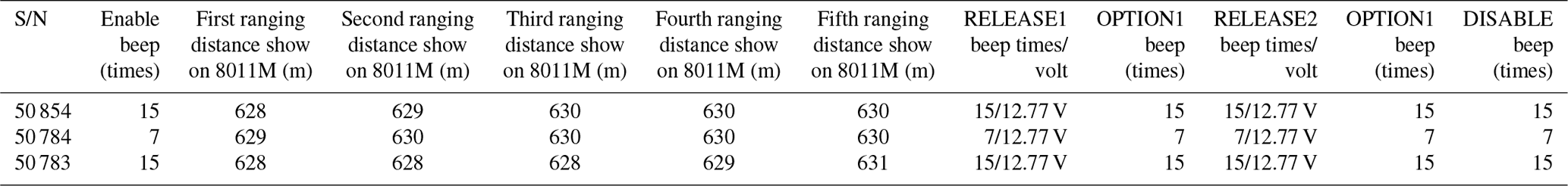
Table 4Example results for the functional test of the acoustic transducer.

Table 5Example results for the functional test of the acoustic controller.
-
Connect the tested transducer and acoustic transceiver via an underwater cable, and place the tested transducer and transceiver at an underwater depth of 1 m.
-
Record the serial numbers of the transducers in a notebook.
-
Send the ENABLE command via the 8011M, and then count the response beeps.
-
Send the RANGE command via the 8011M five times, and record the distance of each ranging.
-
Send the DISABLE command via the 8011M, and then count the response beeps.
-
Replace the transducer, and return to step 2 to repeat the evaluation.
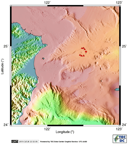
Figure 11A location map showing the Yardbird-BBs and OBEM with triangle and diamond symbols, respectively.
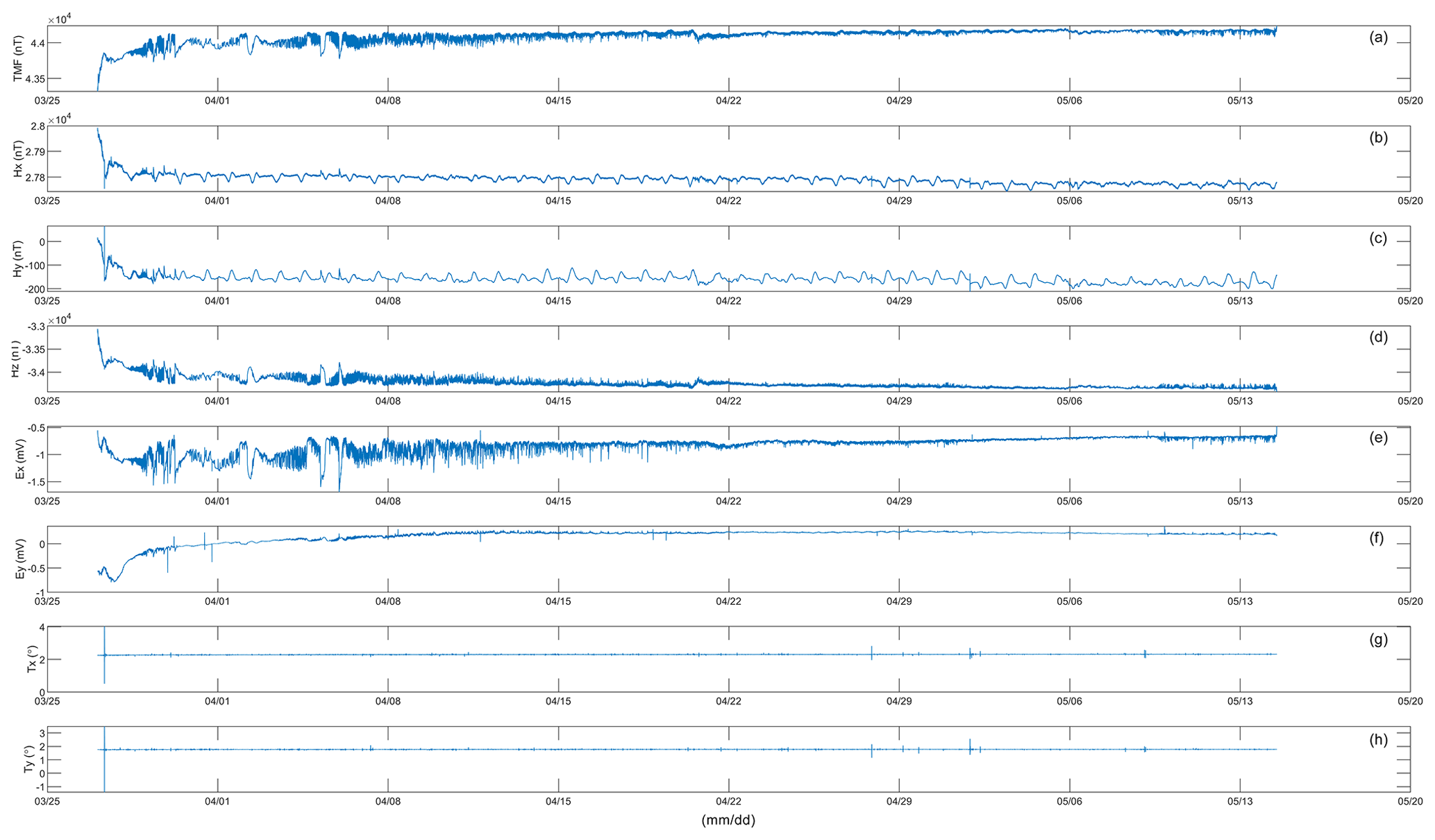
Figure 12The OBEM01 time series data. The panels from top to bottom in the figure show the four magnetic fields (a–d: TMF, HX, HY and HZ), the two electric fields (e, f: EX and EY) and the two inclinations (g, h: TX and TY).
We then checked the acoustic transceivers after all of the transducers were successfully checked; the testing procedure for the acoustic controller is described below. The results are listed in Table 5.
-
Change the acoustic controller, and record its serial number in a notebook.
-
Send the ENABLE command via the 8011M, and then count the response beeps.
-
Send the RANGE command via the 8011M five times, and record the distance of each ranging.
-
Send the RELEASE1 command via the 8011M, and then count the response beeps. Check the voltage between Pin1 and Pin2 of JP2 using a VOM. It should be greater than 12.0 VDC.
-
Send the “OPTION1” command via the 8011M, and then count the response beeps. Check the voltage between Pin1 and Pin2 of JP2 using a VOM. It should be 0 VDC.
-
Send the RELEASE2 command via the 8011M, and then count the response beeps. Check the voltage between Pin3 and Pin4 of JP2 using a VOM. It should be greater than 12.0 VDC.
-
Send the OPTION1 command via the 8011M, and then count the response beeps. Check the voltage between Pin3 and Pin4 of JP2 using a VOM. It should be 0 VDC.
-
Send the DISABLE command via the 8011M, and then count the response beeps.
-
Send the RANGE command via the 8011M; there should be no response from the transceiver.
-
Return to step 1 to repeat the evaluation.
A mercury switch is mounted on the transceiver which when turned off responds with 15 beeps and when turned on responds with seven beeps.

Figure 13Comparison of the OBEM01 and 1802OBS time series data during the two earthquakes. The two earthquakes affected the inclinations. The first and secondary earthquakes occurred at 12:41 and 12:47 UTC, respectively, on 27 April 2018. SH1 and SH2: two horizontal components of the seismic signal; SZ: vertical component of the seismic signal.

Figure 14The variations in PGV, TMF, HY, TX and TY during the first earthquake. The PGV of 2.63 cm s−1 affected the inclinations by 0.601 and 0.404∘ for TX and TY, respectively, and the HY magnetic field had a peak of 100 nT. SH1 and SH2: two horizontal components of the seismic signal; SZ: vertical component of the seismic signal.
We deployed six Yardbird-BBs and one OBEM near a small submarine volcano area in the OT offshore NE Taiwan (Fig. 11) on 26 March 2018 for a submarine observation to evaluate all the OBEM units. All the equipment was successfully recovered after 1 month of deployment. Figure 12 shows the time series of data of OBEM01. The TMF calculated from the three components of the magnetic field varied in the range of 44 100–44 150 nT, which corresponded to the geomagnetic field measured by proton magnetometers in Taiwan. The two horizontal magnetic fields contained significant daily variations. Furthermore, the vibrations of the inclinations were significantly affected by two earthquakes on 27 April 2018 (at 12:41 and 12:47 UTC) consistent with seismic signals of the Yardbird-BBs (Fig. 13). The average magnetic fields of HX, HY, HZ and TMF 2 s prior to the earthquakes (12:41 UTC) were 12 900, 34 300, 24 600 and 44 137 nT, respectively, the average potential fields of EX and EY were −0.79 and −0.149 mV, respectively, and the inclinations of TX and TY were −2.65 and 1.21∘, respectively. These were the averages of the background without earthquakes.
We subtracted the background averages of the magnetic fields and the inclinations to compare the differential during the 12:41 UTC event as shown in Fig. 14. The peak ground motion velocity (PGV) was 2.63 cm s−1 on the SH1 corresponding to inclinations of 0.4 and 0.6∘ for TX and TY with a 100 nT disturbance of HY. There was an insignificant amount of variation in the electric fields. The result shows that the earthquake significantly affected the HY component, whereas HX and HZ components also slightly affected by the earthquake. It could be related to the orientations of the magnetic sensor and the earthquake.
A long-period OBEM acquisition platform to measure magnetic and electrical fields on the seafloor was successfully constructed and evaluated by the OBS R&D team for deployment offshore Taiwan. The power consumption of the OBEM is less than 1 W, which means that the lifetime could be extended up to 300 d with the installation of 108 lithium batteries. We deployed and recovered the OBEM at an underwater depth of 1400 m to acquire the first marine magnetotelluric data offshore NE Taiwan.
Six Yardbird-BBs and one OBEM were deployed near a small submarine volcano area offshore NE Taiwan. The TMF calculated from the three magnetic field components varied in the range of 44 100–44 150 nT, which corresponded to the proton magnetometer measurements of the geomagnetic field in Taiwan. The two horizontal magnetic fields displayed significant daily variations, and the vibrations of the inclinations were significantly affected by the two earthquakes that occurred during the observations. There was an insignificant amount of variation in the electric fields.
Localized microearthquakes affected the disturbances of the magnetic field and inclinations in this study. Therefore, to improve the efficacy of marine geophysical explorations, a platform for multiple underwater measurements is required including an ocean bottom flowmeter, thermometer and absolute pressure gage. We will focus on such developments, in which the evaluated results show that the data logger, flush and radio beacons, EMI filter, and an integrated junction board must be improved in relation to noise levels, cost and convenient maintenance issues in the future.
The data used in the paper can be accessed by contacting the corresponding author.
CRL and CWC wrote the paper with contributions from all authors. KYH primarily provided results on testing and characterizing OBEM performance. The OBEMs presented here were developed at the Taiwan Ocean Research Institute led by YHH under a contract from the National Ocean Taiwan University, Academia Sinica, the National Applied Research Laboratories and the National Taiwan University. PCC, HKC and JPJ designed, constructed, built, assembled and tested infrastructure at the Taiwan Ocean Research Institute used to characterize and document OBEM for this paper. KHC and FSL completed preliminary tests of the OBEM manufacturing process. SL and BYK primarily completed the literature review on the OBEM.
The authors declare that they have no conflict of interest.
We greatly appreciate the crews of R/V OR2 for the field experiments. We also thank 4 years of the Taiwan–German cooperative projects on gas hydrate of NEPII for supporting the funds of the instrument deployment of the OBEMs. We would like to thank the TEC Data Center for proving graphical services. We are also grateful for valuable comments and suggestions of the reviewers.
This research has been supported by the MOST, TAIWAN (grant nos. 101-3113-P-002-013, 102-3113-P-002-005, 103-3113-M-002-004, 104-3113-M-002-004, 105-2116-M-019-001, 106-2116-M-001-008, 106-2116-M-019-003, 107-2116-M-019-006, 108-2116-M-001-012 and 108-2116-M-019-006).
This paper was edited by Valery Korepanov and reviewed by Kai Chen and Denghai Bai.
Bertrand, E., Unsworth, M., Chiang, C. W., Chen, C. S., Chen, C. C., Wu, F., Turkoglu, E., Hsu, H. L., and Hill, G.: Magnetotelluric evidence for thick-skinned tectonics in central Taiwan, Geology, 37, 711–714, 2009.
Bertrand, E. A., Unsworth, M. J., Chiang, C. W., Chen, C. S., Chen, C. C., Wu, F. T., Turkoglu, E., Hsu, H. L., and Hill, G. J.: Magnetotelluric imaging beneath the Taiwan orogen: An arc-continent collision, J. Geophys. Res.-Sol. Ea., 117, B01402, https://doi.org/10.1029/2011JB008688, 2012.
Chiang, C. W., Unsworth, M. J., Chen, C. S., Chen, C. C., Lin, A. T. S., and Hsu, H. L.: Fault zone resistivity structure and monitoring at the Taiwan Chelungpu Drilling Project (TCDP), Terr. Atmos. Ocean Sci., 19, 473–479, 2008.
Chiang, C. W., Chen, C. C., Unsworth, M., Bertrand, E., Chen, C. S., Thong, D. K., and Hsu, H. L.: The deep electrical structure of southern Taiwan and its Tectonic Implications, Terr. Atmos. Ocean Sci., 21, 879–895, 2010.
Chiang, C. W., Chen, C. C., Unsworth, M., Bertrand, E., Chen, C. S., Kieu, T. D., and Hsu, H. L.: Corrigendum to “The deep electrical structure of southern Taiwan and its tectonic implications”, Terr. Atmos. Ocean Sci., 22, 371–371, 2011.
Chiang, C. W., Hsu, H. L., and Chen, C. C.: An investigation of the 3D electrical resistivity structure in the Chingshui geothermal area, NE Taiwan, Terr. Atmos. Ocean Sci., 26, 269–281, 2015.
Ellis, M., Evans, R. L., Hutchinson, D., Hart, P., Gardner, J., and Hagen, R.: Electromagnetic surveying of seafloor mounds in the northern Gulf of Mexico, Mar. Pet. Geol., 25, 960–968, 2008.
Evans, R. L., Hirth, G., Baba, K., Forsyth, D., Chave, A., and Mackie, R.: Geophysical evidence from the MELT area for compositional controls on oceanic plates, Nature, 437, 249–252, 2005.
Kasaya, T. and Goto, T.: A small ocean bottom electromagnetometer and ocean bottom electrometer system with an arm-folding mechanism, Explor. Geophys., 40, 41–48, 2009.
Key, K.: Marine Electromagnetic Studies of Seafloor Resources and Tectonics, Surv. Geophys., 33, 135–167, 2012.
Kuo, B. Y., Wang, C. C., Lin, S. C., Lin, C. R., Chen, P. C., Jang, J. P., and Chang, H. K.: Shear-wave splitting at the edge of the Ryukyu subduction zone, Earth Planet. Sc. Lett., 355, 262–270, 2012.
Kuo, B. Y., Webb, S. C., Lin, C. R., Liang, W. T., and Hsiao, N. C.: Removing infragravity-wave-induced noise from Ocean-Bottom Seismographs (OBS) data deployed offshore of Taiwan, B. Seismol. Soc. Am., 104, 1674–1684, 2014.
Kuo, B. Y., Crawford, W. C., Webb, S. C., Lin, C. R., Yu, T. C., and Chen, L. W.: Faulting and hydration of the upper crust of the SW Okinawa Trough during continental rifting: Evidence from seafloor compliance inversion, Geophys. Res. Lett., 42, 4809–4815, 2015.
Utada, H.: Electromagnetic exploration of the oceanic mantle, P. Jpn. Acad. B-Phys., 91, 203–222, 2015.