A Tethered Air Blimp (TAB) for observing the microclimate over a complex terrain

This study presents the first environmental monitoring field campaign of a newly developed Tethered Air Blimp (TAB) system to investigate the microclimate over a complex terrain. The use of a tethered balloon in complex terrains such as mines and tailings ponds is novel and the focus of the present study. The TAB system was fully developed and launched at a mining facility in northern Canada in May 2018. This study describes the key design features, the sensor payload on board, calibration, and the observations made by the TAB system. The system measured meteorological conditions including components of wind velocity vector, temperature, relative humidity, and pressure over the first few tens of metres of the atmospheric boundary layer. The measurements were made at two primary locations in the facility: (i) near a tailings pond and (ii) in a mine pit. TAB measured the dynamics of the atmosphere at different diurnal times (e.g. day versus night) and locations (near a tailings pond versus inside the mine). Such dynamics include mean and turbulence statistics pertaining to flow momentum and energy, and they are crucial in the understanding of emission fluxes from the facility in future studies. In addition, TAB can provide boundary conditions and validation datasets to support mesoscale dispersion modelling or computational fluid dynamics simulations for various transport models.

1 Introduction

The atmospheric boundary layer (ABL) is the lowest portion of the air near the Earth's surface that responds to surface processes in 1 h or less (Stull, 1988; Aliabadi, 2018). The understanding of the atmospheric turbulent processes governing the transfer of heat, moisture, and momentum in the surface layer is of practical importance for many applications such as weather and climate prediction, pollution dispersion, and urban air quality studies (Zilitinkevich and Baklanov, 2002; Pichugina et al., 2008; Aliabadi et al., 2016b, c). Most of the research in atmospheric turbulence has been focused on relatively smooth terrain and horizontally homogeneous environments mainly due to the limitation in the availability of adequate observation platforms and difficulty in acquiring data from the complex environments. However, the study of the ABL and surface–atmosphere interaction over complex terrain is very important for many applications. Surface heterogeneity can cause horizontal gradients of momentum or temperature, and it can influence or complicate the horizontal and vertical transport mechanisms, for instance, driven by slope flows or thermals (Mahrt and Vickers, 2005; Medeiros and Fitzjarrald, 2014). In addition, model parameterizations of turbulent processes established for atmospheric flows over smooth and homogeneous surfaces often fail when applied over heterogeneous and complex terrains (Roth, 2000).

1.1 Literature review

Two types of ABL observations of the meteorological parameters are key: atmospheric properties and Earth surface properties (Mäkiranta et al., 2011; Manoj et al., 2014). Conventional techniques measuring the atmospheric properties such as remote sensing (e.g. satellite, radars (radio detection and ranging), lidars (light detection and ranging), sodars (sonic detection and ranging), radiometers) and in situ measurements (meteorological masts, aircraft, or sounding balloons) are widely used for observing variables such as wind, humidity, and temperature (Pichugina et al., 2008; Legain et al., 2013; Aliabadi et al., 2016b, 2019). The main disadvantages of such conventional techniques are the low frequency of turbulence measurements (sodars and lidars), cost (aircraft and satellites), difficulty of navigation (sounding balloons), intermittency of observation (aircraft, sounding balloons, and non-geostationary satellites), low spatial resolution (geostationary satellites), and limited spatial coverage (meteorological towers) (Fernando and Weil, 2010; Medeiros and Fitzjarrald, 2014). In addition, measuring the surface layer within the ABL poses a serious challenge to aircraft that cannot fly at altitudes lower than 150 m in many jurisdictions for safety reasons (Mayer et al., 2012).

Airborne systems are increasingly being used for atmospheric measurements (Martin et al., 2011; Palomaki et al., 2017), although recently their use is being regulated more restrictively. For instance, rotary or fixed-wing drones are not permitted to fly in complex environments such as busy urban areas and airports. On the other hand, tethered-balloon-based atmospheric measurement techniques have been used widely for obtaining the turbulence structure as well as the mean vertical profiles of the ABL meteorological variables in complex environments (Thompson, 1980). One of the main advantages of a tethered-balloon system is its ability to profile a significant portion of the planetary boundary layer starting from the surface, which is not possible or economical by ground-based or aircraft-based atmospheric measurement techniques (Egerer et al., 2019). The use of ultrasonic anemometers in tethered balloons has been reported in many studies (Canut et al., 2016). In comparison, one of the disadvantages of Pitot tubes is their inability to measure the low wind speeds. So they require a fast flying probe which cannot fly in a complex environment for safety and logistic reasons. Ultrasonic anemometers, on the other hand, are popular because of their continuous measurement characteristics, high accuracy, and ability to be levitated to measure low velocities.

Tethered-balloon-borne atmospheric turbulence measurements have a long history of observations over land (Smith, 1961) and sea (Thompson, 1972) to measure fluxes of heat and moisture at heights up to a few hundred metres. The most notable tethered-balloon systems deployed collected data in campaigns in the late 1960s and 1970s including the Barbados Oceanographic and Meteorological Experiment (BOMEX) (Davidson, 1968; Garstang and La Seur, 1968; Friedman and Callahan, 1970), the Joint Air-Sea Interaction (JASIN) experiment (Pollard, 1978), and the Global Atmospheric Research Programme (GARP) Atlantic Tropical Experiment (GATE) (Berman, 1976). In BOMEX, a tethered-balloon system was operated from the deck, which measured temperature, wind, and humidity continuously, at different levels in the range of 0 to 600 m in the ocean area north and east of the island of Barbados. In JASIN, tethered balloons were used to measure the structure of ABL to understand the air–sea interaction in the North Atlantic. In the recent past, tethered-balloon systems have been used in Boundary-Layer Late Afternoon and Sunset Turbulence (BLLAST) field campaign that was conducted in southern France (Lothon et al., 2014). Canut et al. (2016) used an ultrasonic anemometer mounted on a tethered-balloon system for turbulent flux and variance measurements. Egerer et al. (2019) used the BELUGA (Balloon-bornE moduLar Utility for profilinG the lower Atmosphere) tethered-balloon system for profiling the lower Atmosphere by turbulence and radiation measurements in the Arctic. Tethered balloons have also been used to perform Earth surface thermal imaging in complex open-pit mines and the surrounding complex terrain (Byerlay et al., 2020).

The interactions between meteorology and topography are very important because of the energy exchanges at the land surface–atmosphere interface. The micrometeorological patterns are greatly influenced by the geographical features such as the morphology of the Earth's surface (e.g. valleys, flat terrains, and Earth depression), composition, structure, synoptic events, and the seasonal weather variation (Clements et al., 2003; Whiteman et al., 2004). The meteorological patterns of flat terrains are different from that of an Earth depression (Clements et al., 2003; Whiteman et al., 2004; Nahian et al., 2020). Meteorological processes inside the Earth depressions and their surroundings are complex. There are multiple studies (Clements et al., 2003; Whiteman et al., 2004, 2008) carried out in natural Earth depressions, which observed that nighttime micrometeorology inside the depression shows different circulation patterns, reduced advective transfer with outside of the depression, reduced turbulent sensible heat flux at the bottom, reduced slope flows, and formation of weak and intermittent turbulent jets on the depression walls near the ground. It is also observed that, at night, a temperature stratification occurs inside the depression with a cool pool of air at the bottom and a warm pool of air near the edge of the depression (Clements et al., 2003; Whiteman et al., 2004, 2008; Lehner et al., 2016). There are not many studies focusing on the meteorology of the open-pit mines to see if they feature similar meteorological conditions to those of the natural Earth depressions. The dynamic nature of the industrial operations (rapid landscape transformation by mining) changes the thermodynamic and aerodynamic properties of the exposed surfaces (e.g. albedo, emissivity, aerodynamic roughness length scale). Also, anthropogenic heat release due to use of equipment and the presence of water bodies such as tailings ponds create a complex system to study.

1.2 Objectives

There are only a few comprehensive field studies that focus on the ABL over a mine environment, while the structure of ABL in an orographically complex terrain such as a mine can be complicated (Rotach and Zardi, 2007; Medeiros and Fitzjarrald, 2014, 2015). In the surface layer, flows are highly influenced by the terrain geometry, while Coriolis effects have still negligible influences (Arroyo et al., 2014).

The Tethered Air Blimp (TAB), developed by the authors, is a mobile sensing platform for the investigation of surface layer within ABL overcoming some of the limitations mentioned in the literature review. TAB is lifted by the buoyancy force and requires no propulsion power for navigation compared to drones. This allows turbulence measurements over long periods without disturbing the surrounding air. It provides accurate in situ measurements unlike remote sensing technologies such as lidars, sodars, and satellites. It is safer to operate at low altitudes compared to aircraft. It can be controlled and redeployed using a tether, unlike radiosondes, and it is very cost effective. TAB can collect high-time-resolution observations of the weather to characterize the turbulence properties in low altitudes in almost all weather conditions. In the case of extreme wind, TAB can still be used with the help of additional stabilizing tethers (up to three). The variables it measures include components of wind velocity vector, temperature, relative humidity, and pressure.

TAB observations can be utilized in numerous ways. Atmospheric dynamics as measured by TAB can determine transport mechanisms that drive emission fluxes (Steudler et al., 1991). Factors such as mean wind speed, atmospheric diffusion coefficient, and thermal stability greatly influence emission fluxes (Bowden et al., 1993), all of which are measured by TAB. It can also provide boundary conditions and validation datasets to support ABL simulations of climate, weather, and dispersion using highly parameterized models, computational fluid dynamics models, or mesoscale models (Bueno et al., 2012; Holnicki and Nahorski, 2015; Aliabadi et al., 2017; Nahian et al., 2020).

1.3 Structure of the paper

The structure of the paper is organized as follows. Section 2 briefly describes the TAB system and the sensors' payload. Calibration experiments are explained in Sect. 3. Section 4 presents field experiments and results of the environmental monitoring campaign where TAB was used in a complex mining facility. Conclusions and future recommendations are provided in Sect. 5.

2 TAB specification

TAB consists of a helium balloon, a controlling tether, a tether reel, and a gondola platform housing the sensors. The payload in the gondola platform is comprised of microclimate sensors, such as a mini weather station, a thermal camera, and a flight controller. The payload items can be altered to use different sensors suitable for a particular application. The thermal imaging system design and usage is fully described in a study by Byerlay et al. (2020) and not discussed here.

2.1 Envelope and platform

The balloon envelope is manufactured by Aero Drum Ltd. (https://www.rc-zeppelin.com/, last access: 15 February 2019). It is an ellipsoid made out of polyurethane with dimensions of 2.8 m × 2.8 m × 1.9 m providing axisymmetric aerodynamic stability. The envelope is filled with up to 8 m³ of balloon-grade helium capable of lifting 5 kg of payload although at least 1.5 kg of surplus lift is recommended for stable performance. The polyurethane envelope provides a good seal and results in only up to a maximum 0.5 % volume helium loss per day, enabling the system to be used up to 24 h before a helium recharge is necessary. The tethers enable deployment of the balloon at a location of interest while controlling the ascend or descend rate of the balloon manually. The horizontal range of the TAB is within 50 m of launch point as the balloon system is controlled by multiple tethers on the ground. A close-up of the TAB system during sampling and a system schematic can be seen in Fig. 1.

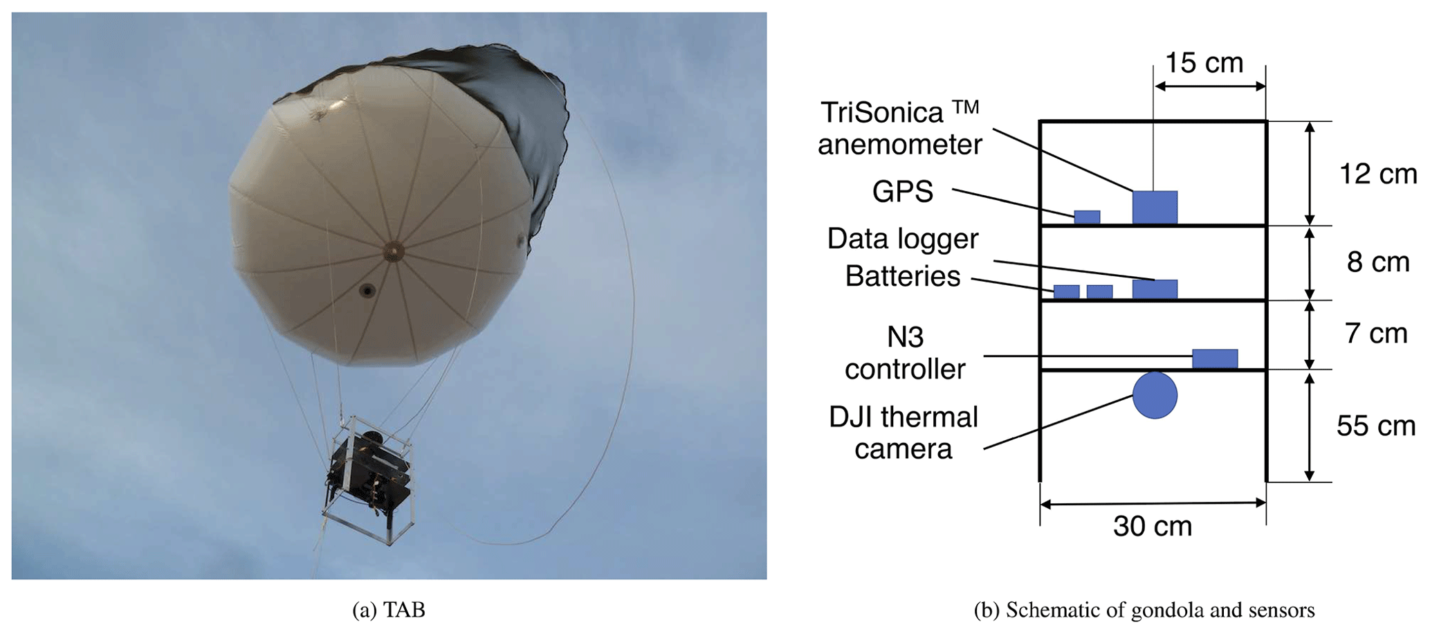
Figure 1 Close-up of the TAB system during sampling and the schematic of the TAB gondola with all the sensors.

The acting forces on the system are (1) the lift force due to the helium-filled balloon, (2) the force of gravity, (3) the tension forces due to the tethers, and (4) the drag force due to the wind. In the absence of the drag force, the remaining forces are acting in the vertical direction and the system ascends up or down, but the presence of the drag force displaces the system in the horizontal direction. At all times, these forces are balanced so that the TAB is in a quasi-stationary state.

The balloon is equipped with a net that helps facing the balloon against the main wind direction at any moment. The net guides the air on one side, and the pressure force stops the balloon from rotating. In the case of wind direction changing, the pressure force builds up on the net, creating a torque around the centre of rotation that repositions the balloon facing the main wind. Up to three tethers are used to control the balloon to help with stabilizing the system, especially during high winds associated with convective boundary layers. The tethers, however, impose extra weight on the system so that the vertical range of the system reduces when three tethers are used as opposed to one or two tethers.

Figure 2a shows the balloon operation in an unstable atmosphere with high winds when three tethers are used to stabilize it. A sudden drag force on the gondola may drive the system out of its stable position momentarily. Hence, it may affect the quality of measurements by creating instabilities. Such a phenomenon can be prevented by deploying extra tethers connecting the gondola directly to ground operators. The tension in these tethers balances the sudden drag force exerted on the system. This arrangement places the gondola in a quasi-stationary state in the air that indeed helps the stability of measurement in gusty conditions. Figure 2b shows the balloon operation in a stable atmosphere with low winds when only two tethers are used to stabilize it. A T connector connects the balloon to the gondola using tethers allowing the gondola to hang freely while minimizing the pitch-and-roll angles to result in better measurements from a levelled gondola.

Figure 2 TAB at different atmospheric stability conditions tethered with two or three stabilization ropes in the mining facility.

2.2 Mini weather station

The TriSonica™ Mini weather station is an ultrasonic anemometer manufactured by Anemoment™ and is mounted onto the gondola of TAB (https://www.anemoment.com/, last access: 10 January 2019). The Mini weather station is ideal for applications that require a miniature, lightweight, and low velocity anemometer, and it is suitable particularly for airborne systems. It has a measurement path length of 35 mm and a weight of 50 g. The light weight makes it an ideal candidate to use with the TAB system. It can measure the components of the wind velocity vector, air temperature, relative humidity, and the barometric pressure at a sampling rate up to 10 Hz. The open path provides the least possible distortion of the wind field. Its design with four measurement pathways provides a redundant measurement and the path with the most distortion is removed from the calculations to provide accurate wind measurements. It is also equipped with a compass and a tilt sensor. Because of its low power consumption (only 30 mA at 12 V), it is highly power efficient and can record data for hours on a single battery charge.

A data logger by Applied Technologies Inc. (http://www.apptech.com/, last access: 10 March 2019) is used as the data synchronization and data collection device for the TriSonica™ Mini weather station. This data logger records the measurements on an SD card on board that can be retrieved after every flight. In addition, the TriSonica™ Mini can be monitored or programmed using serial communication via the data logger. The TriSonica™ Mini weather station and the data logger are powered using a 12 V lithium–polymer (LiPo) battery.

The anemometer measures wind speed in the range 0–30 m s⁻¹ at a resolution of 0.1 m s⁻¹. The accuracy of the measurement is ±0.1 m s⁻¹ (0–15 m s⁻¹) or ±2 % (15–30 m s⁻¹). Wind direction is measured at a resolution of 1^∘ and an accuracy of ±1^∘. Vertical winds are measured appropriately if the approach elevation angle is within ±30^∘, a condition that is typically met under calm wind conditions over smoothly varying topography. Temperature is measured in a range from −25 ^∘C to +80 ^∘C with a resolution of 0.1 ^∘C and an accuracy of ±2 ^∘C. Pressure is measured in the range 50–115 Pa with an accuracy of ±1 kPa. The tilt sensor measures the pitch and roll with an accuracy of ±0.5^∘. The compass measures the magnetic heading with an accuracy of ±5^∘.

The TriSonica™ Mini wind measurements are referenced to a frame with fixed coordinate axis directions along east, north, and normal to the Earth's surface using rotation matrices. This was made possible by use of the heading, roll, and pitch angles measured by the TriSonica™ Mini. The sensor has a coordinate system in which the +x axis is from local north N_T of the sensor to local south S_T, the +y axis is from local east E_T to local west W_T, and the +z axis is downward, i.e. toward the Earth's surface. This local coordinate system is right handed. Likewise, the velocities measured by the sensor are positive along these axes. Let the sensor's coordinate system be shown by x_T, y_T, and z_T and the corresponding velocities be shown by U_T, V_T, and W_T. The sensor measures heading h, positive clockwise with respect to magnetic north N_M. It measures the pitch angle p, which is a positive downward rotation of x_T about y_T, and the roll angle r, which is positive downward rotation of y_T about x_T. The goal is to transform this coordinate system, by means of rotation matrices, to align with a reference frame of the Earth with x_F pointing from west to east, y_F pointing from south to north, and z_F pointing away upward from the surface of the Earth. This coordinate system is also right handed. The resulting velocity transformation will provide U_F, V_F, and W_F in the final coordinate system.

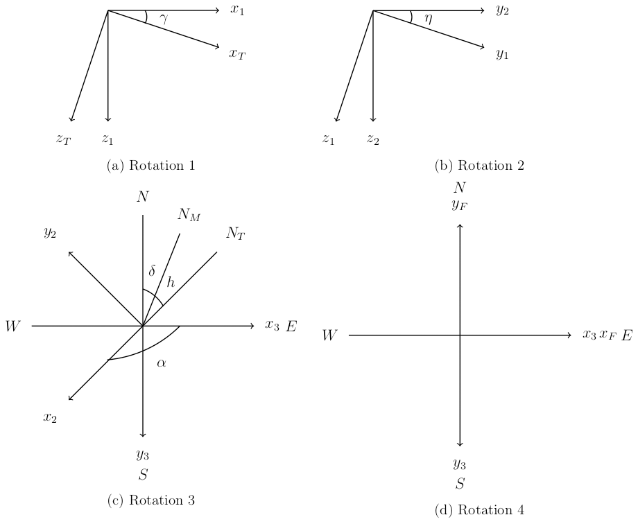
Figure 3 (a) Rotation about y_T by γ=p; figure viewed normal to the y_T=y₁ axis; (b) rotation about x₁ by η=r; figure viewed normal to the x₁=x₂ axis; (c) rotation about z₂ by $\mathit{\alpha }=(\mathit{\delta }+h+\mathrm{90})\mathit{\%}\mathrm{360}$; figure viewed normal to the z₂=z₃ axis; (d) rotation about x₃ by π; figure viewed normal to the z₃ axis.

As depicted in Fig. 3a, the first rotation should be about the local y_T axis by an angle γ=p. This transformation results in an intermediate coordinate system x₁, y₁, and z₁ so that the x₁ axis will be aligned with the horizon, i.e. parallel to the Earth's surface. Note that the figure is viewed normal to y_T=y₁ and that in this coordinate system z₁ is still not yet normal to the Earth's surface and that y₁ is still not yet aligned with the horizon. This transformation is given by

$$\begin{array}{}\text{(1)}& \left[\begin{array}{c}{x}_{\mathrm{1}}\\ y_{\mathrm{1}}\\ z_{\mathrm{1}}\end{array}\right]=\left[\begin{array}{ccc}\cos \left(\mathit{\gamma }\right)& \mathrm{0}& \sin \left(\mathit{\gamma }\right)\\ \mathrm{0}& \mathrm{1}& \mathrm{0}\\ -\sin \left(\mathit{\gamma }\right)& \mathrm{0}& \cos \left(\mathit{\gamma }\right)\end{array}\right]\left[\begin{array}{c}{x}_{\mathrm{T}}\\ y_{\mathrm{T}}\\ z_{\mathrm{T}}\end{array}\right]=R_{y,\mathit{\gamma }}\left[\begin{array}{c}{x}_{\mathrm{T}}\\ y_{\mathrm{T}}\\ z_{\mathrm{T}}\end{array}\right].\end{array}$$

As depicted in Fig. 3b, the second rotation should be about x₁ axis by an angle η=r. This transformation results in another intermediate coordinate system (x₂, y₂, and z₂), so that now the y₂ axis will be aligned with the horizon, i.e. parallel to the Earth's surface. Note that the figure is viewed normal to x₁=x₂ and that in this coordinate system z₂ is normal to the Earth's surface. This transformation is given by

$$\begin{array}{}\text{(2)}& \left[\begin{array}{c}{x}_{\mathrm{2}}\\ y_{\mathrm{2}}\\ z_{\mathrm{2}}\end{array}\right]=\left[\begin{array}{ccc}\mathrm{1}& \mathrm{0}& \mathrm{0}\\ \mathrm{0}& \cos \left(\mathit{\eta }\right)& -\sin \left(\mathit{\eta }\right)\\ \mathrm{0}& \sin \left(\mathit{\eta }\right)& \cos \left(\mathit{\eta }\right)\end{array}\right]\left[\begin{array}{c}{x}_{\mathrm{1}}\\ y_{\mathrm{1}}\\ z_{\mathrm{1}}\end{array}\right]=R_{x,\mathit{\eta }}\left[\begin{array}{c}{x}_{\mathrm{1}}\\ y_{\mathrm{1}}\\ z_{\mathrm{1}}\end{array}\right].\end{array}$$

As depicted in Fig. 3c, the third rotation should be about z₂ axis by an angle $\mathit{\alpha }=(\mathit{\delta }+h+\mathrm{90})\mathit{\%}\mathrm{360}$, where δ is the magnetic declination of the Earth, which is dependent on a specific latitude and longitude. For the current site, δ=13.5^∘. Here, the modulus with 360 is taken since the heading angle can vary from 0 to 360^∘. This transformation results in another intermediate coordinate system (x₃, y₃, and z₃), so that now the y₃ axis will be aligned from north to south and the x₃ axis will be aligned from west to east. Note that the figure is viewed normal to z₂=z₃. This transformation is given by

$$\begin{array}{}\text{(3)}& \left[\begin{array}{c}{x}_{\mathrm{3}}\\ y_{\mathrm{3}}\\ z_{\mathrm{3}}\end{array}\right]=\left[\begin{array}{ccc}\cos \left(\mathit{\alpha }\right)& -\sin \left(\mathit{\alpha }\right)& \mathrm{0}\\ \sin \left(\mathit{\alpha }\right)& \cos \left(\mathit{\alpha }\right)& \mathrm{0}\\ \mathrm{0}& \mathrm{0}& \mathrm{1}\end{array}\right]\left[\begin{array}{c}{x}_{\mathrm{2}}\\ y_{\mathrm{2}}\\ z_{\mathrm{2}}\end{array}\right]=R_{z,\mathit{\alpha }}\left[\begin{array}{c}{x}_{\mathrm{2}}\\ y_{\mathrm{2}}\\ z_{\mathrm{2}}\end{array}\right].\end{array}$$

As depicted in Fig. 3d, the fourth and final rotation should be about x₃ axis by an angle π. This transformation results in the final coordinate system with x_F, y_F, and z_F axes, which point west to east, south to north, and normal upward from the Earth's surface, respectively. This transformation is given by

$$\begin{array}{}\text{(4)}& \left[\begin{array}{c}{x}_{\mathrm{F}}\\ y_{\mathrm{F}}\\ z_{\mathrm{F}}\end{array}\right]=\left[\begin{array}{ccc}\mathrm{1}& \mathrm{0}& \mathrm{0}\\ \mathrm{0}& \cos \left(\mathit{\pi }\right)& -\sin \left(\mathit{\pi }\right)\\ \mathrm{0}& \sin \left(\mathit{\pi }\right)& \cos \left(\mathit{\pi }\right)\end{array}\right]\left[\begin{array}{c}{x}_{\mathrm{3}}\\ y_{\mathrm{3}}\\ z_{\mathrm{3}}\end{array}\right]=R_{x,\mathit{\pi }}\left[\begin{array}{c}{x}_{\mathrm{3}}\\ y_{\mathrm{3}}\\ z_{\mathrm{3}}\end{array}\right].\end{array}$$

In compressed form, the entire coordinate transformation can be shown as follows. This immediately implies a similar transformation for the measured velocities by the sensor:

$$\begin{array}{}\text{(5)}& \left[\begin{array}{c}{x}_{\mathrm{F}}\\ y_{\mathrm{F}}\\ z_{\mathrm{F}}\end{array}\right]=R_{x,\mathit{\pi }}{R}_{z,\mathit{\alpha }}{R}_{x,\mathit{\eta }}{R}_{y,\mathit{\gamma }}\left[\begin{array}{c}{x}_{\mathrm{T}}\\ y_{\mathrm{T}}\\ z_{\mathrm{T}}\end{array}\right],\end{array}$$

$$\begin{array}{}\text{(6)}& \left[\begin{array}{c}{U}_{\mathrm{F}}\\ V_{\mathrm{F}}\\ W_{\mathrm{F}}\end{array}\right]=R_{x,\mathit{\pi }}{R}_{z,\mathit{\alpha }}{R}_{x,\mathit{\eta }}{R}_{y,\mathit{\gamma }}\left[\begin{array}{c}{U}_{\mathrm{T}}\\ V_{\mathrm{T}}\\ W_{\mathrm{T}}\end{array}\right].\end{array}$$

3 Calibration experiments

3.1 Wind velocity calibration

To calibrate wind measurements of TriSonica™ Mini, multiple experiments were conducted using the University of Guelph's wind tunnel, which is an open circuit tunnel designed for turbulent boundary layer research. The cross-sectional area is 1.2 m × 1.2 m. The tunnel is 10 m long. The tunnel's air speed is controlled by a gauge that sets the fan speed. The tunnel achieves wind speeds up to 10 m s⁻¹. The turbulence intensity is typically less than 2 % if no roughness blocks are placed upstream of the flow. The Reynolds number of flow in the tunnel varies between 150 000 and 1 100 000. Considering the size of the wind tunnel, it is capable of generating eddies as large as its physical dimensions.

The performance of the gondola (or the effects of the frame on TriSonica™ Mini measurements) in reading the mean and turbulence statistics of the flow field was studied with respect to an R.M. Young 81000 anemometer, which was already calibrated, and used for cross comparison to derive the calibration coefficients for the TriSonica™ Mini using line fits. By adding multiple degrees of freedom, the setup for this test was designed to further simulate the gondola's movements in the real atmosphere. The gondola was attached to the ceiling of the tunnel with two tethers (featuring the tethers to the balloon) and a single tether to the bottom floor of the tunnel (resembling the ground operator). Now, the gondola faces the main flow (as it does in the real atmosphere), but it has some degrees of freedom to slightly wobble. The azimuth angle, elevation angle, and wind levels were changed, independently, to derive calibration coefficients for both mean and turbulence statistics as measured by the TriSonica™ Mini and calibrated against the R.M. Young 81000 sensor. Both sensors were set up at similar airflow conditions while wind speed was varied at few wind levels in the range 2–10 m s⁻¹. At each wind speed level, data recording continued for 5 min. Each recording was time averaged to calculate mean and turbulence statistics.

In this study, the velocity along the x, y, and z directions is denoted by U, V, and W. Further, Reynolds decomposition is used to express each velocity component as the sum of the time-averaged and fluctuating components: $U=\stackrel{\mathrm{‾}}{U}+u$, $V=\stackrel{\mathrm{‾}}{V}+v$, and $W=\stackrel{\mathrm{‾}}{W}+w$, where the over-lined quantities are time averages and lower case quantities are instantaneous fluctuations. Furthermore, variance and covariance of the fluctuations are represented by $\stackrel{\mathrm{‾}}{u^{\mathrm{2}}}$, $\stackrel{\mathrm{‾}}{uw}$, etc. The wind tunnel calibration equations obtained are used for correcting the field measurement data from the TAB.

Even though we calibrated the wind measurement on the gondola system, our wind tunnel facility is too small and cannot enclose the size of the balloon for an overall system calibration. When we analysed the potential flow distortion around the balloon in an analytical way, the results indicated that the measurement of the vertical wind velocity component is not influenced by the presence of the balloon, but the horizontal wind velocity component can be enhanced by up to ∼20 %. Certainly, the potential flow assumption is not valid for the atmosphere, but the analytical calculation provides an idea about how much wind measurement can be influenced by the presence of the balloon.

3.2 Temperature calibration

Temperatures measured by TriSonica™ Mini are calibrated with respect to a Campbell Scientific HMP60 sensor (https://www.campbellsci.com/, last access: 10 January 2019). The latter collected minute-averaged temperatures, to which the TriSonica™ Mini temperatures were also averaged and compared. The calibration experiment was carried out under a set of weather conditions to cover a wide range of temperatures outdoors. In this study, temperature measurements were converted to potential temperatures using the pressure measurements. Likewise, Reynolds averaging was used to decompose the potential temperature as the sum of the time-averaged and fluctuating components: $\mathrm{\Theta }=\stackrel{\mathrm{‾}}{\mathrm{\Theta }}+\mathit{\theta }$.

4 Field experiments and results

The TAB system was launched at a mining facility in northern Canada (above 56^∘ N) for an environmental monitoring field campaign in May 2018. A schematic of the mining facility can be seen in Fig. 4. The depth of the mine is approximately 100 m.

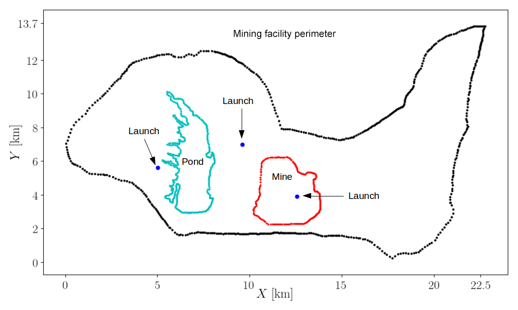
Figure 4 A schematic of the mining facility; the black dots represent the outline of the entire facility. The green dots represent the outline of the tailings pond, and the red dots represent the outline of the mine. The blue dots are the balloon launch locations.

TAB flew for 56 h while collecting data. The objectives of the measurements were to determine dynamics of the atmosphere at different diurnal times (e.g. day versus night) and locations (near a tailings pond versus inside the mine). Such dynamics determine the transport of greenhouse gases (GHGs) and therefore emission fluxes. Measurements of the GHG fluxes were not the objective of this paper and will be addressed elsewhere.

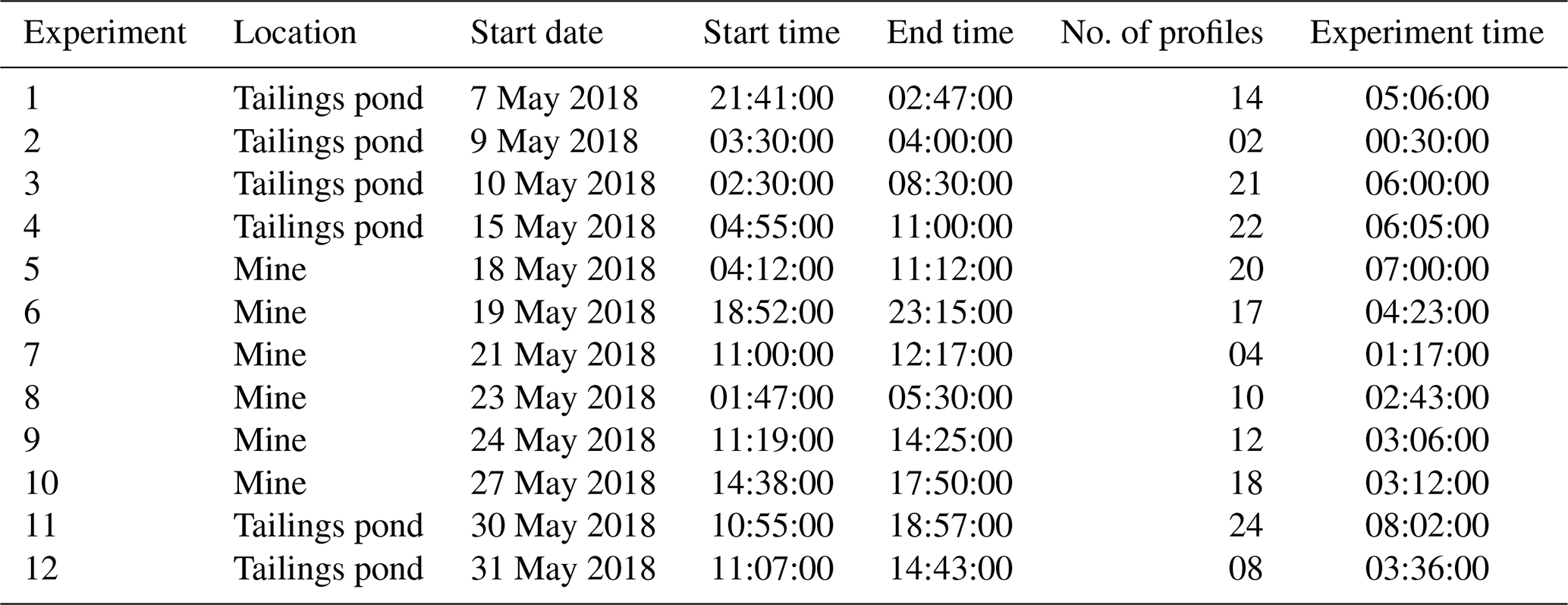
Surface-level transport mechanisms strongly depend on atmospheric dynamics. Factors such as wind speed, atmospheric diffusion coefficient, and thermal stability greatly influence emission fluxes. As a result, the particular focus of this study was measurement of surface-level meteorology in the lowest 200 m altitude. The launch details are summarized in Table 1.

Table 1 TAB launch details; times are in Local Daylight Time (LDT).

Vertical transport of momentum and heat are predominant processes within the surface layer of the ABL (Businger et al., 1971), and probing of the vertical fluxes of momentum and heat from wind velocity vector and temperature profile measurements can be achieved using TAB. Turbulence kinetic energy is one of the key measures of turbulence in the atmosphere, as it controls the vertical and horizontal mixing (Lenschow et al., 1980; Svensson et al., 2011; Shin et al., 2013; Canut et al., 2016). It is also used for the parameterization of small-scale turbulent transport processes, such as vertical fluxes, when the smaller-scale motions are not modelled directly (Aliabadi et al., 2018). The equation that represents turbulence kinetic energy is

$$\begin{array}{}\text{(7)}& k={\displaystyle \frac{\mathrm{1}}{\mathrm{2}}}\left(\stackrel{\mathrm{‾}}{u^{\mathrm{2}}}+\stackrel{\mathrm{‾}}{v^{\mathrm{2}}}+\stackrel{\mathrm{‾}}{w^{\mathrm{2}}}\right),\end{array}$$

where $\stackrel{\mathrm{‾}}{u^{\mathrm{2}}}$, $\stackrel{\mathrm{‾}}{v^{\mathrm{2}}}$, and $\stackrel{\mathrm{‾}}{w^{\mathrm{2}}}$ are the variance of turbulent velocity fluctuations along the three coordinate system axes. Another parameter that expresses the relative roles of shear and buoyancy in the production/consumption of turbulence kinetic energy is the Obukhov length L, which is used to define the atmospheric stability condition (Golder, 1972). The equation for the Obukhov length is

$$\begin{array}{}\text{(8)}& L=-{\displaystyle \frac{\stackrel{\mathrm{‾}}{\mathrm{\Theta }}{u}_{*}^{\mathrm{3}}}{g\mathit{\kappa }\stackrel{\mathrm{‾}}{w\mathit{\theta }}}},\end{array}$$

where $\stackrel{\mathrm{‾}}{\mathrm{\Theta }}$ is the mean potential temperature, κ=0.4 is the von Kármán constant, g is the acceleration due to gravity, $\stackrel{\mathrm{‾}}{w\mathit{\theta }}$ is the vertical kinematic sensible heat flux, and u_* is the friction velocity:

$$\begin{array}{}\text{(9)}& u_{*}=\sqrt[\mathrm{4}]{\left({\stackrel{\mathrm{‾}}{u^{\prime }{w}^{\prime }}}^{\mathrm{2}}+{\stackrel{\mathrm{‾}}{v^{\prime }{w}^{\prime }}}^{\mathrm{2}}\right)},\end{array}$$

where $\stackrel{\mathrm{‾}}{u^{\prime }{w}^{\prime }}$ and $\stackrel{\mathrm{‾}}{v^{\prime }{w}^{\prime }}$ are the vertical kinematic momentum fluxes in the x and y directions, respectively. We used the hypsometric equation to calculate the altitude of the measurement above surface (Stull, 2015):

$$\begin{array}{}\text{(10)}& z_{\mathrm{2}}-z_{\mathrm{1}}\approx a\stackrel{\mathrm{‾}}{T_{\mathrm{v}}}\ln \left({\displaystyle \frac{P_{\mathrm{1}}}{P_{\mathrm{2}}}}\right),\end{array}$$

where P₁ and P₂ are the pressure measurement at two altitudes (z₁ and z₂). The system measured pressure in mBar although the equation is insensitive to the units of pressure. The unit of altitude is m. $\stackrel{\mathrm{‾}}{T_{\mathrm{v}}}$ is the average virtual temperature between altitudes z₁ and z₂. The constant $a=R_d/g$ is equal to 29.3 m K⁻¹ (Stull, 2015). Given the uncertainty of temperature and pressure measurement, the uncertainty of altitude measurement is estimated as 1.2 m (Byerlay et al., 2020).

4.1 Sampling time

TAB measured wind speed, the turbulence kinetic energy, variance, and fluxes for both momentum and heat rigorously. Each balloon launch lasted approximately 15–30 min, while the tether was carefully controlled to obtain a profile with constant ascent and descent rates. The sampling time for calculating the mean and turbulence quantities was 3 min, while typically it is 10 to 30 min for flux tower measurements (Aliabadi et al., 2019). For turbulence statistics, the time series is first detrended to ensure that background weather variations that have inherently very large timescales and length scales are filtered out without influencing the turbulence statistics calculations. It is known that finite time sampling, instead of ensemble averaging, will introduce random and systematic errors in the prediction of turbulence statistics such as variance and fluxes (Lenschow et al., 1994). While random errors could result in overprediction or underprediction of turbulence statistics, the systematic errors always underpredict the magnitude of the turbulence statistics. These errors have been reported in an aircraft campaign to be anywhere in the range 10 % to 90 % of the measured value (Aliabadi et al., 2016b). While repeated measurements, increasing the averaging time, and detailed error analysis are possible to eliminate such errors from predictions, the focus of this study was not to investigate errors associated with finite sampling time. Nevertheless, operating the TAB involves a delicate choice of the sampling time. On the one hand, short sampling times have inherent large errors but provide profiles at high vertical resolutions. On the other hand, long sampling times have inherent small errors but provide profiles at low vertical resolutions.

4.2 Diurnal variation in wind speed and turbulence statistics

It was observed that both wind speed (Fig. 5) and turbulence kinetic energy (Fig. 6) exhibited a significant diurnal variation, indicating calm conditions at night and in the early morning, when atmospheric diffusion coefficient is low, and gusty conditions during mid-afternoon when the atmospheric diffusion coefficient is high. When calculating statistical percentiles, the data are combined over all altitudes and aggregated for both the mine and tailings pond locations.

Similar diurnal variations can be also observed in the case of other turbulence statistics such as friction velocity u_*, Obukhov length L, vertical kinematic sensible heat flux $\stackrel{\mathrm{‾}}{w\mathit{\theta }}$, potential temperature variance $\stackrel{\mathrm{‾}}{{\mathit{\theta }}^{\mathrm{2}}}$, and vertical velocity variance $\stackrel{\mathrm{‾}}{w^{\mathrm{2}}}$ (Fig. 7). Note that L was limited to ±500 m for post-processing of the measured data. The measurement of weak turbulence in the nocturnal boundary layer is also very important, as it leads to weak turbulent dispersion and large accumulation of heat or atmospheric constituents in the lower part of the stable boundary layer (Mahrt and Vickers, 2003, 2006). Periods of strong stability with intermittent turbulence can also occur in the nocturnal boundary layer (Businger et al., 1971; Mahrt, 1999).

Figure 5 Diurnal variation of wind speed; at each hour, observations are plotted using statistical percentiles (5th, 25th, 50th, 75th, and 95th); times are in LDT.

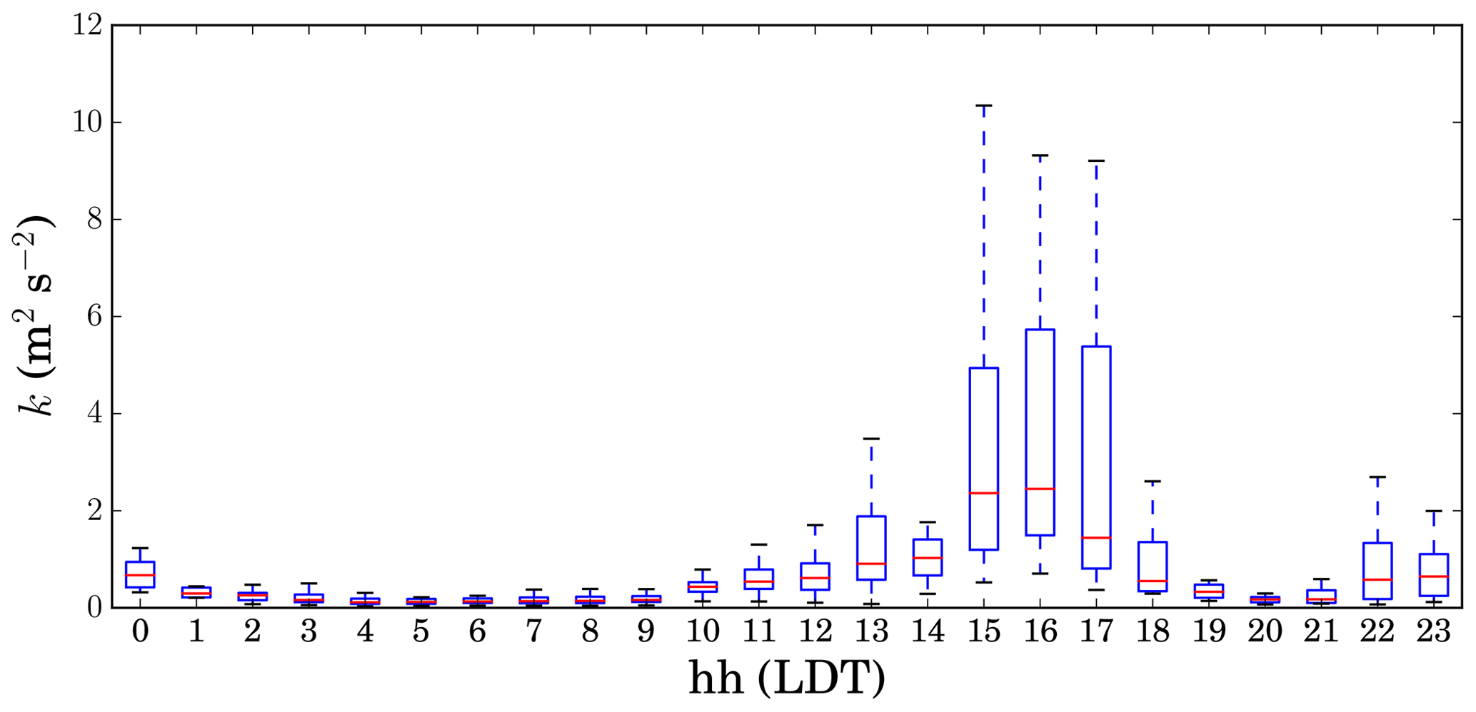
Figure 6 Diurnal variation of turbulence kinetic energy; at each hour, observations are plotted using statistical percentiles (5th, 25th, 50th, 75th, and 95th); times are in LDT.

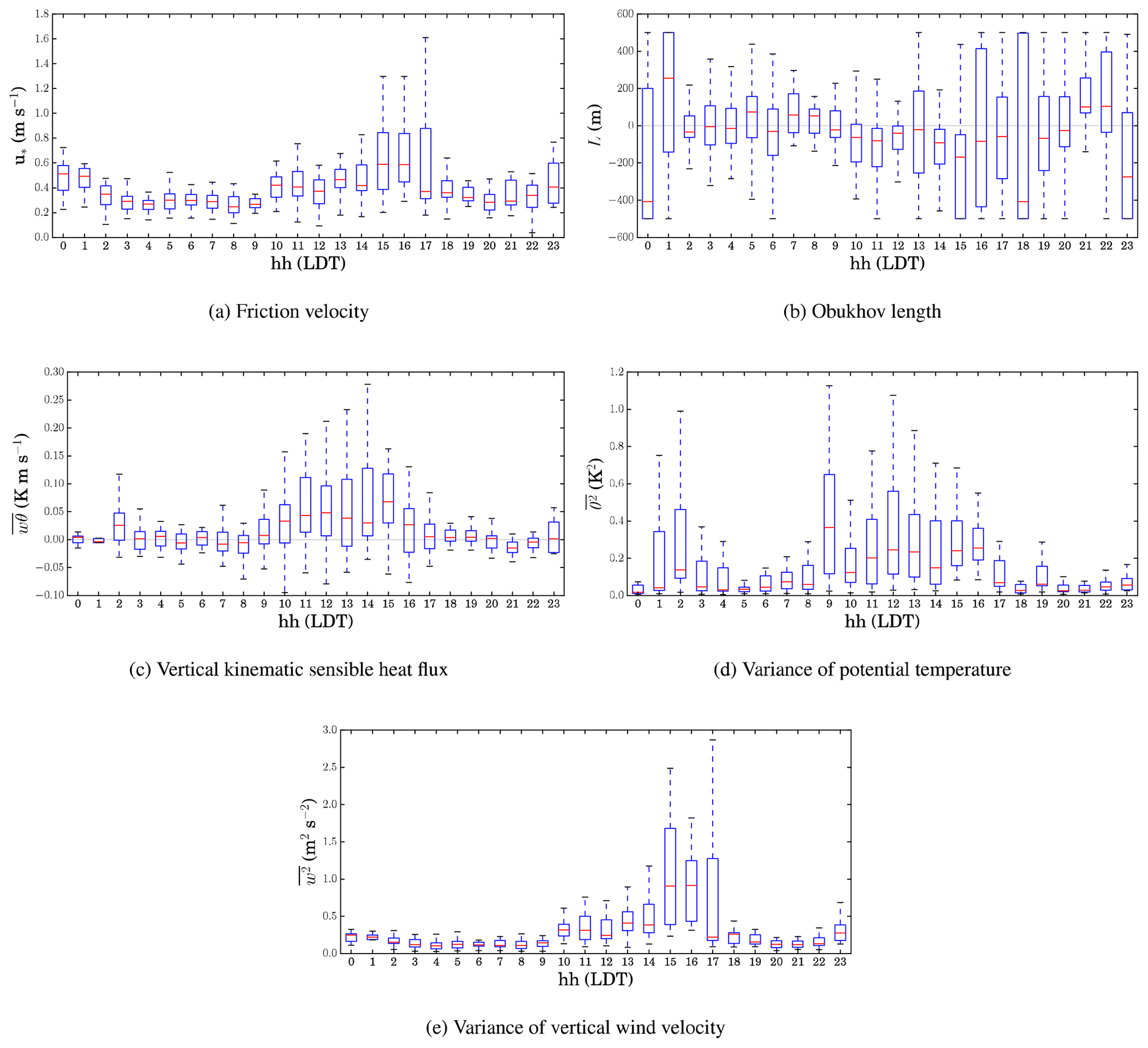
Figure 7 Diurnal variation of different turbulence statistics; at each hour, observations are plotted using statistical percentiles (5th, 25th, 50th, 75th, and 95th); times are in LDT.

4.3 Vertical variation of mean and turbulence statistics

Figure 8 shows the vertical profiles of turbulence statistics for different diurnal periods (4 h intervals) of the day. The 50th percentiles are shown for all observations. Data are binned in 20 m height intervals. The vertical structure of the atmosphere near the surface can be understood while analysing the turbulence kinetic energy k, friction velocity u_*, Obukhov length L, vertical kinematic sensible heat flux $\stackrel{\mathrm{‾}}{w\mathit{\theta }}$, variance of potential temperature $\stackrel{\mathrm{‾}}{{\mathit{\theta }}^{\mathrm{2}}}$, and variance of vertical wind velocity $\stackrel{\mathrm{‾}}{w^{\mathrm{2}}}$.

It is noteworthy that maximum flight altitude is usually lower under windy conditions; therefore, most profiles obtained under windy conditions at midday are shorter than those obtained under calm conditions at night and early mornings. It is observed that in the surface layer within ABL the highest gradients of turbulence properties occur at the lowest 100 m. This statement must be considered with caution. Certainly, it is only valid for the short length scales and timescales of fluctuation considered as a result of the 3 min time averaging. The diurnal variation of turbulence statistics is clear from the plots. The magnitudes for most statistics (except for L) are greatest during the midday time interval at 12:00–16:00 Local Daylight Time (LDT) due to gusty conditions, while the magnitudes are smallest during the nighttime and early-morning time interval (04:00–08:00 LDT) associated with calm conditions. This also implies confidence in the measurement of velocity fluctuation covariance. The vertical kinematic sensible heat flux $\stackrel{\mathrm{‾}}{w\mathit{\theta }}$ is negative during nighttime but positive during daytime. The variance of potential temperature $\stackrel{\mathrm{‾}}{{\mathit{\theta }}^{\mathrm{2}}}$ is not strictly diminished under calm nighttime conditions. This can be interpreted as the presence of differential near-surface horizontal gradients of temperature due to thermal structures caused by the surface. It is expected that such gradients must exist because of the heterogeneity of land surface and anthropogenic activities in such a complex terrain of a mining facility.

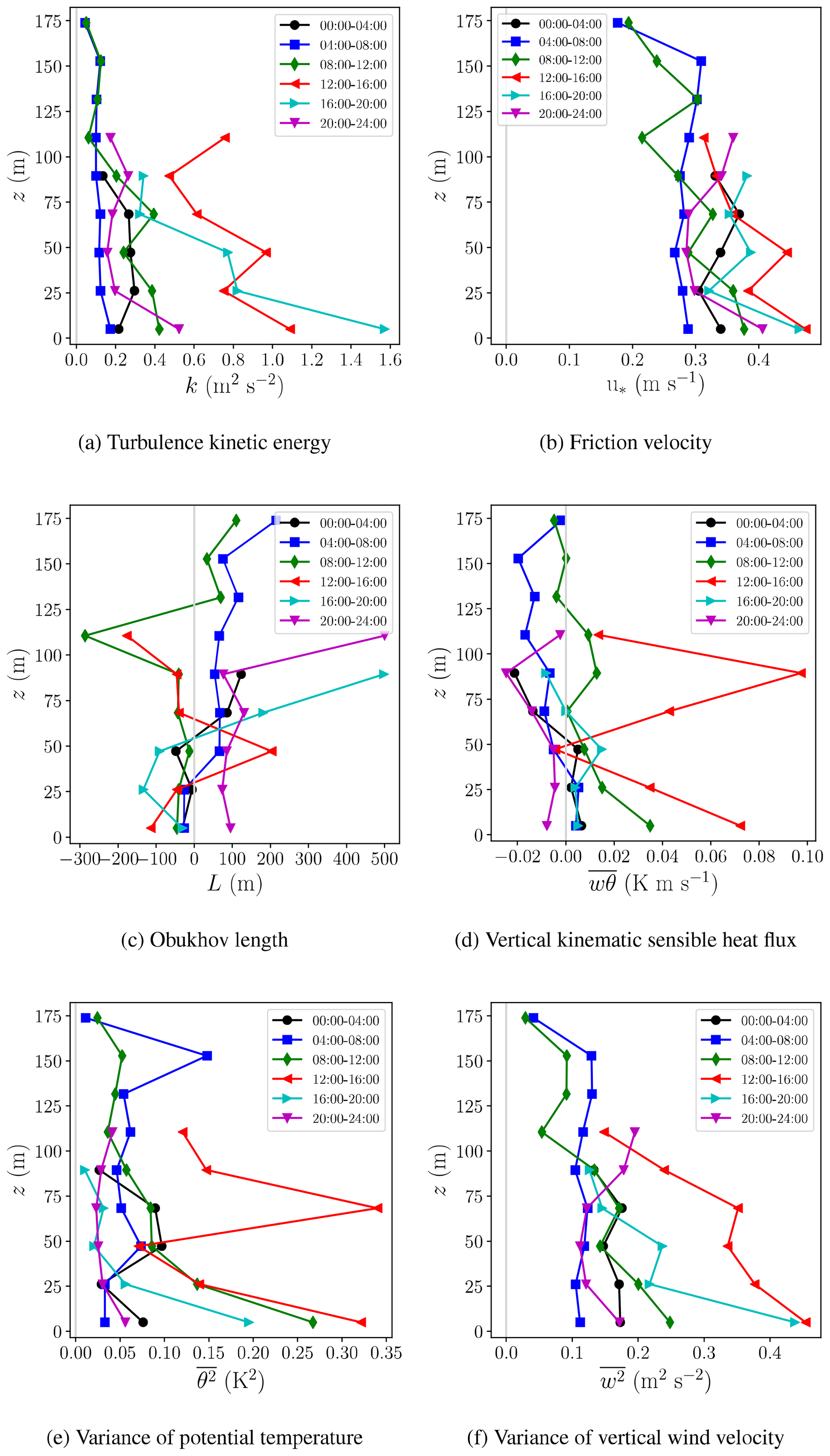
Figure 8 Vertical profiles of different turbulence statistics for different diurnal time periods (4 h intervals) of the day; times are in LDT.

4.4 Variation of thermal stability and wind speed as a function of diurnal time

The atmospheric dynamical condition can be described using two parameters: (1) wind speed and (2) thermal stability. The wind speed determines mechanical advection and usually the higher the wind speed is, the greater the atmospheric transport and diffusion coefficient will be. Thermal stability determines the buoyant transport in the vertical direction in the atmosphere. Thermal stability is reported using various methods employing variables such as (i) the vertical gradients of the potential temperature (Liu and Liang, 2010), (ii) the bulk Richardson number (Mahrt, 1981; Aliabadi et al., 2016a), or (iii) the Monin–Obukhov length (Obukhov, 1971; Wilson, 2008).

If vertical gradients of the potential temperature or the bulk Richardson number are positive, the atmosphere is stable and the buoyant transport is suppressed. This occurs during the nights and early mornings. If the vertical gradients of the potential temperature and bulk Richardson number are negative, the atmosphere is unstable and buoyant transport is enhanced. This occurs during the mid-afternoons. If the vertical gradients of potential temperature and bulk Richardson number are close to zero, the atmosphere is neutral, in which case buoyant transport is still present but weak.

Figures 9 and 10 show evidence for the variation of vertical profiles of potential temperature and wind speed as a function of diurnal time and height, respectively. The profiles for the thermally stable condition on 7 and 8 May 2018 were measured on the west side of the tailings pond, which is a flat area, while the profiles for the thermally unstable condition on 30 May 2018 were measured on the east side of the tailings pond, which is a sloped area. Here, the data are statistically processed in 3 min intervals, such that a median is calculated for each 3 min interval. Since observations for these plots are not aggregated over many days, the height interval is not binned.

The effect of thermal stability on profiles of the potential temperature is clear. While the profiles of wind speed on the west of the tailings pond show the onset of the logarithmic law; the profiles of wind speed on the east side of the tailings pond show evidence of higher wind speeds at altitudes 10–40 m above ground. These are downslope winds given that the measured local wind direction was from the north. The presence of this jet near the surface is in agreement with drainage flows upstream of the depression measured by Lehner et al. (2016) in the Arizona Meteor Crater experiment (their Fig. 7) and downslope flows measured by Clements et al. (2003) in Utah's Peter Sinks (their Fig. 12). Controlled by topography, land cover, soil moisture, radiative exchange, local shading, and surface energy budget, such slope flows are hypothesized to form under fair weather conditions as a result of heating of atmospheric layers during daytime and cooling during nighttime (Hari Prasad et al., 2017).

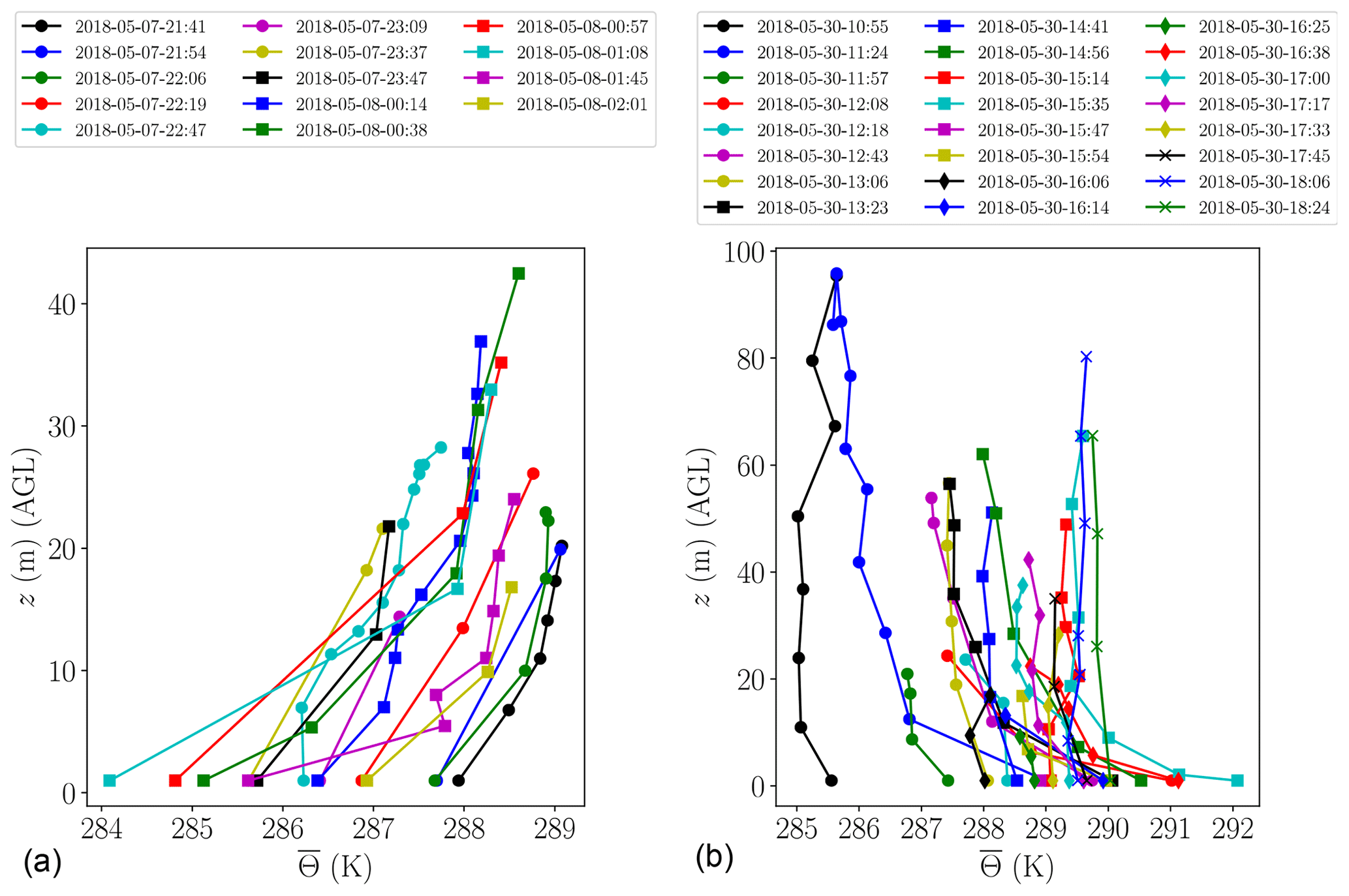
Figure 9 Vertical profiles of potential temperature on 7, 8 and 30 May 2018. (a) Thermally stable condition at night and in the early morning when the gradients are positive near the surface; (b) thermally unstable condition at midday when the gradients are negative near the surface; times are in LDT.

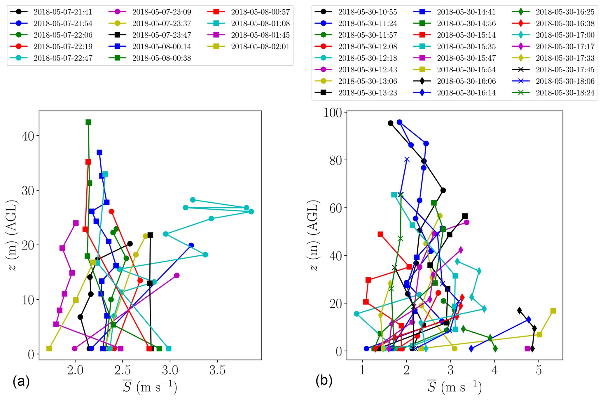
Figure 10 Vertical profiles of wind speed on 7, 8 and 30 May 2018. (a) Thermally stable condition at night and early morning, (b) thermally unstable condition at midday; times are in LDT.

4.5 Atmospheric dynamical condition

As shown in Fig. 11, all observations were used to determine the atmospheric dynamical condition on a two-dimensional map consisting of thermal stability, i.e. bulk Richardson number Ri_b, and mean wind speed $\stackrel{\mathrm{‾}}{S}$. Here, the bulk Richardson number is defined as

$$\begin{array}{}\text{(11)}& {\mathit{Ri}}_{\mathrm{b}}={\displaystyle \frac{gH}{({\stackrel{\mathrm{‾}}{S}}_{\mathrm{H}}-{\stackrel{\mathrm{‾}}{S}}_{\mathrm{S}}{)}^{\mathrm{2}}}}{\displaystyle \frac{{\stackrel{\mathrm{‾}}{\mathrm{\Theta }}}_{\mathrm{H}}-{\stackrel{\mathrm{‾}}{\mathrm{\Theta }}}_{\mathrm{S}}}{{\stackrel{\mathrm{‾}}{\mathrm{\Theta }}}_{\mathrm{A}}}},\end{array}$$

where g is gravitational acceleration, H is the maximum altitude for each launch, ${\stackrel{\mathrm{‾}}{S}}_{\mathrm{H}}$ is mean horizontal wind speed at maximum altitude, ${\stackrel{\mathrm{‾}}{S}}_{\mathrm{S}}$ is mean horizontal wind speed near the surface, ${\stackrel{\mathrm{‾}}{\mathrm{\Theta }}}_{\mathrm{H}}$ is mean potential temperature at maximum altitude, ${\stackrel{\mathrm{‾}}{\mathrm{\Theta }}}_{\mathrm{S}}$ is mean potential temperature near the surface, and ${\stackrel{\mathrm{‾}}{\mathrm{\Theta }}}_{\mathrm{A}}$ is mean potential temperature for the entire launch.

The frequency plot shows the most frequent status of the atmosphere by providing a normalized count of each pair of observed Ri_b and $\stackrel{\mathrm{‾}}{S}$, while the colour plot shows the median value for turbulence kinetic energy k given as a function of each pair of observed Ri_b and $\stackrel{\mathrm{‾}}{S}$. It is found that the atmosphere spends a considerable amount of time under near-neutral and stable conditions during nights and early mornings, where Ri_b≥0, possibly with the same likelihood of unstable state during midday, where Ri_b<0. The colour plot for turbulence kinetic energy shows that the highest values are observed under near-neutral conditions, where Ri_b∼0 and mean wind speed is high such that $\stackrel{\mathrm{‾}}{S}>\mathrm{5}$ m s⁻¹. A few spurious high frequencies of observations are detected for very large Richardson numbers (Ri_b∼10) and very low wind speeds ($\stackrel{\mathrm{‾}}{S}$ ∼ 1–2 m s⁻¹). These are likely due to the inability of TAB to detect mean wind speed gradients under calm conditions. These plots demonstrate that the atmosphere in the surface layer has preferred states. For instance, it was never observed to be very stable and gusty at the same time.

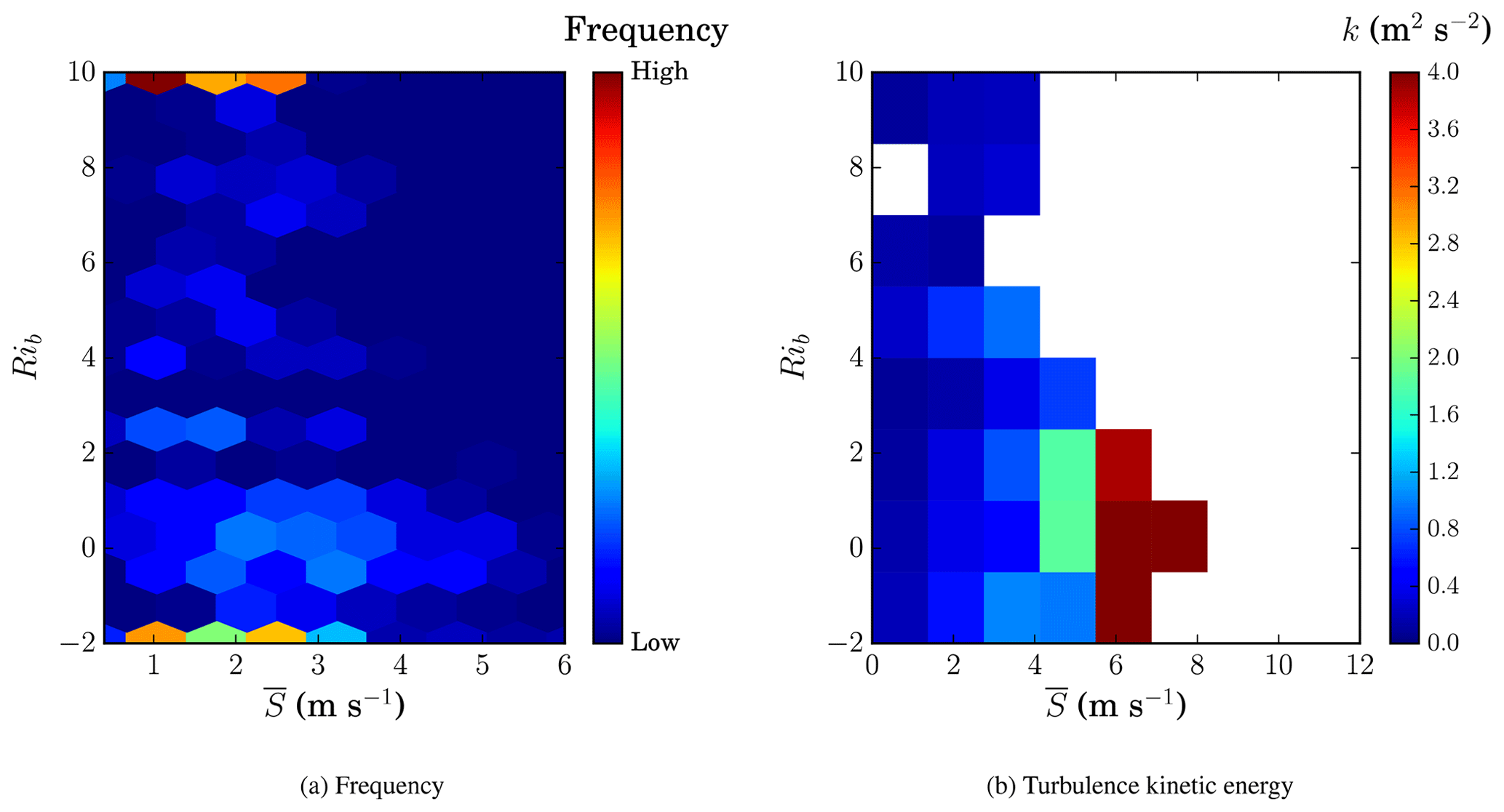
Figure 11 (a) Frequency plot of atmospheric dynamical condition as a function of bulk Richardson number Ri_b and mean wind speed $\stackrel{\mathrm{‾}}{S}$; (b) turbulence kinetic energy k as a function of the same variables.

4.6 Comparison between the mine and the tailings pond

Almost the same number of hours were spent measuring the surface layer at the mine and near the tailings pond using TAB. The measurements attempted to cover a 24 h time period in 3–4 d so that TAB would capture the diurnal variations completely. Note that due to logistical difficulties, it was impossible to measure the surface layer in either location for 24 h continuously. The base location for the launches at the mine was approximately 100 m below grade and at the centre of the mine, while the base locations near the tailings pond were on the west and east sides. We have compared the diurnal variations for various surface layer variables between the mine and near the tailings pond observations. These include the mean horizontal wind speed, turbulence kinetic energy, friction velocity, Obukhov length, vertical kinematic sensible heat flux, variance of vertical velocity vector, and variance of potential temperature. We have also compared the atmospheric dynamical condition in terms of the bulk Richardson number and mean wind speed. The idea behind this comparison was to quantify any differences in surface layer variables as a result of terrain complexity and land use.

4.6.1 Comparison of diurnal variation of turbulence properties

TAB captured the diurnal variation of mean and turbulence statistics in the mine as well as near the tailings pond. In Figs. 12 and 13, we plot the diurnal variations for the mine in red and near the tailings pond in blue. It is observed that, for both in the mine and near the tailings pond, all the turbulence statistics exhibit a significant diurnal variation, indicating calm conditions at nights and early mornings, when the atmospheric diffusion coefficient is low, and gusty conditions in the mid-afternoons when the atmospheric diffusion coefficient is high. The data are aggregated for all altitudes.

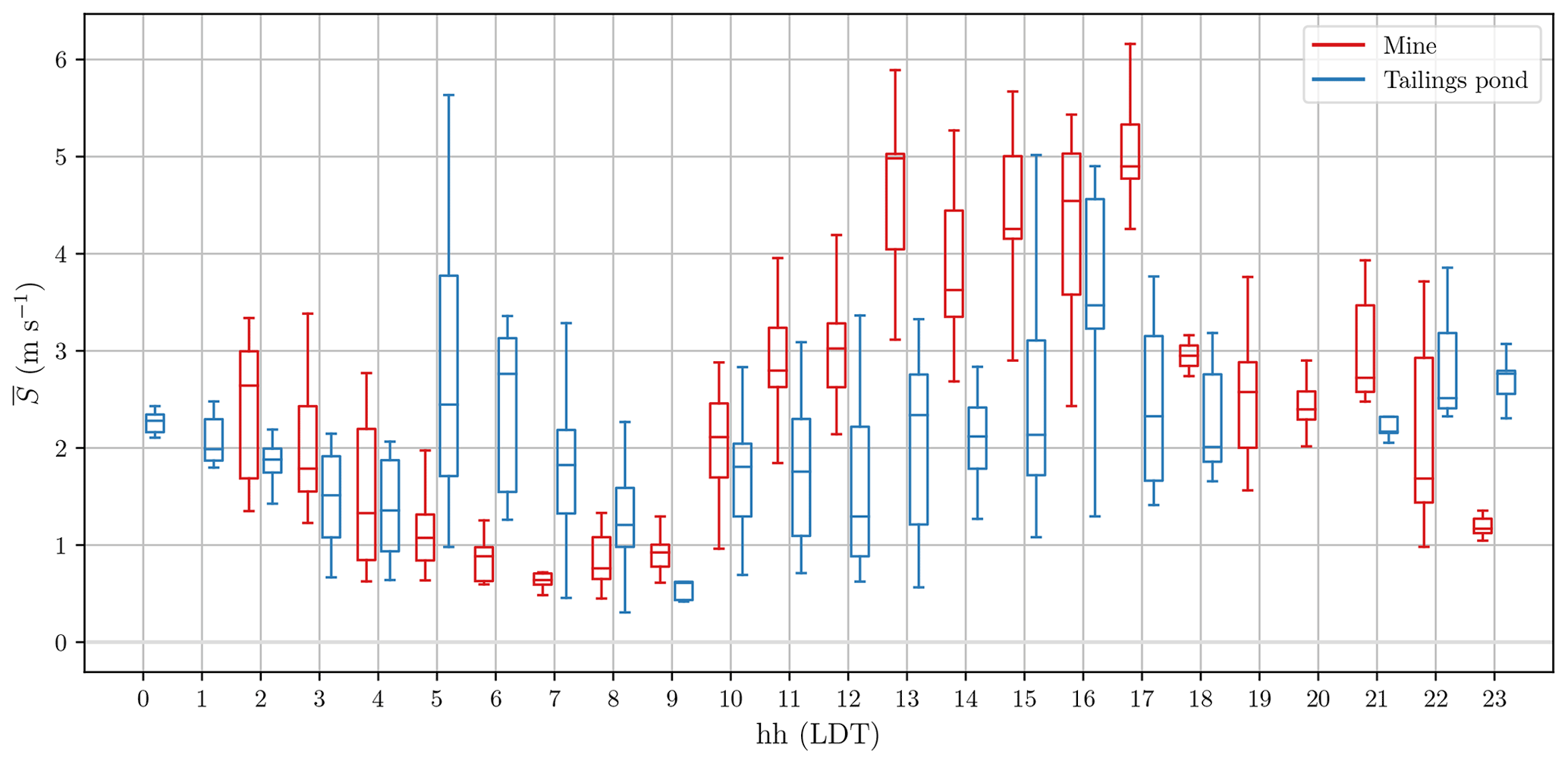
Figure 12 Diurnal variation of mean wind speed; at each hour, observations are plotted using statistical percentiles (5th, 25th, 50th, 75th, and 95th); times are in LDT.

Figure 13 Diurnal variation of different mean and turbulence statistics; at each hour, observations are plotted using statistical percentiles (5th, 25th, 50th, 75th, and 95th); times are in LDT.

There are subtle differences between observations in the mine and near the tailings pond. The trends in mean wind speed $\stackrel{\mathrm{‾}}{S}$, turbulence kinetic energy k, friction velocity u_*, and vertical velocity variance $\stackrel{\mathrm{‾}}{w^{\mathrm{2}}}$ suggest that the mine experiences calm conditions during early morning hours, i.e. from 05:00 to 07:00 LDT, when the atmospheric stability is at its maximum, while at the same time near the tailings pond, higher mean wind speed and turbulence kinetic energy are observed. During early afternoons and under unstable conditions, i.e. from 15:00 to 17:00 LDT, near the tailings pond, lower mean wind speed, turbulence kinetic energy, friction velocity, and vertical velocity variance are observed in comparison to the mine. Even though day-to-day variations of meteorological conditions may contribute to this, there is evidence that such features can also result from terrain complexity and land surface heterogeneity. A modelling study of the same mining facility predicted lower-magnitude winds inside the mine pit, compared to higher-magnitude winds near the tailings pond, during thermally stable conditions, while higher-magnitude winds were predicted inside the mine pit, compared to lower-magnitude winds near the tailings pond, during thermally unstable conditions (Fig. 7 in Nahian et al., 2020). In that study, such a difference was explained considering two mechanisms: net radiation heat transfer between the Earth's surface and the sky, and the heat capacity of the Earth's surface. The Earth's surface always emits longwave radiation upward to the atmosphere and space, yet during the unstable conditions this loss of longwave radiation from the surface is dominated by incoming shortwave (solar) radiation. Given the low heat capacity of the land, this results in warm surface temperatures during the unstable condition and cool surface temperatures during the stable condition. For the tailings pond, given the higher heat capacity, the temperature variation exhibits a lower-amplitude diurnal cycle. This results in warmer water temperatures during stable conditions and cooler water temperatures during the unstable conditions compared to the surrounding land surface temperatures. Hence, in thermally stable hours, the tailings pond surface exhibits a warmer temperature compared to the surrounding areas (and vice versa during the thermally unstable hours). Such thermal gradients can cause differences in wind speed, such that higher surface temperatures enhance convective boundary layers and increase wind speeds, while lower surface temperatures suppress convective boundary layers and reduce wind speed. The formation of a cold and calm pool of air during stable conditions in the natural Earth depressions has also been reported by experimental measurements (Clements et al., 2003; Whiteman et al., 2004, 2008; Lehner et al., 2016).

As far as the vertical kinematic sensible heat flux $\stackrel{\mathrm{‾}}{w\mathit{\theta }}$ and variance of potential temperature $\stackrel{\mathrm{‾}}{{\mathit{\theta }}^{\mathrm{2}}}$ are concerned, the mine measurements show more positive values compared to the measurements near the tailings pond in most diurnal hours (except for hours corresponding to operation staff shift change around 06:00 and 18:00 LDT). This was expected particularly during the early afternoons and under unstable conditions, i.e. from 15:00 to 17:00 LDT. However, in fact, the mine measurements also show positive vertical heat flux and higher potential temperature variance from 02:00 to 03:00 LDT compared to measurements near the tailings pond. This is in contrast to the expectations when comparing the results to the measurements of the natural depressions of the Earth, most of which report reduced vertical kinematic sensible heat flux under stable conditions (Clements et al., 2003; Whiteman et al., 2004, 2008; Lehner et al., 2016). The difference here arises from the fact that excavation activities using heavy machinery is very active in the mine all the time, including during the stable conditions, possibly explaining the higher values of heat flux and potential temperature variance under most stability conditions (except for hours corresponding to operation staff shift change around 06:00 and 18:00 LDT). There is also evidence using thermal imaging of the same facility that mine surface temperatures are higher than the surroundings during many diurnal times (Fig. 7 in Byerlay et al., 2020). Given that the Obukhov length is negatively and inversely proportional to the vertical kinematic sensible heat flux, the mine measurements show more negative values compared to the measurements near the tailings pond although Obukhov length is also proportional to the friction velocity cubed, so the distinction is less clear between the mine and tailings pond measurements of the Obukhov length.

4.6.2 Comparison of atmospheric dynamical condition

Figure 14 shows the frequency plots of atmospheric dynamical condition as a function of the bulk Richardson number Ri_b and mean wind speed $\stackrel{\mathrm{‾}}{S}$ in the mine and near the tailings pond separately. It is very difficult to report statistically significant changes between the two plots; however, some distinctions can be pointed out. For the case of the tailings pond, a cluster of measurements can be spotted for positive bulk Richardson numbers between 3 and 9, while for the case of the mine, such a cluster of measurements is not so evident. This suggests that overall the atmospheric surface layer inside the mine is more thermally unstable. This is consistent with the observation of high positive magnitude for the vertical kinematic sensible heat flux $\stackrel{\mathrm{‾}}{w\mathit{\theta }}$ for mine measurements compared to the tailings pond measurements. Again, the frequency plots should be read with care at Ri_b∼10 due to the lack of a reliable TAB predictions for vertical mean wind speed gradients under calm conditions.

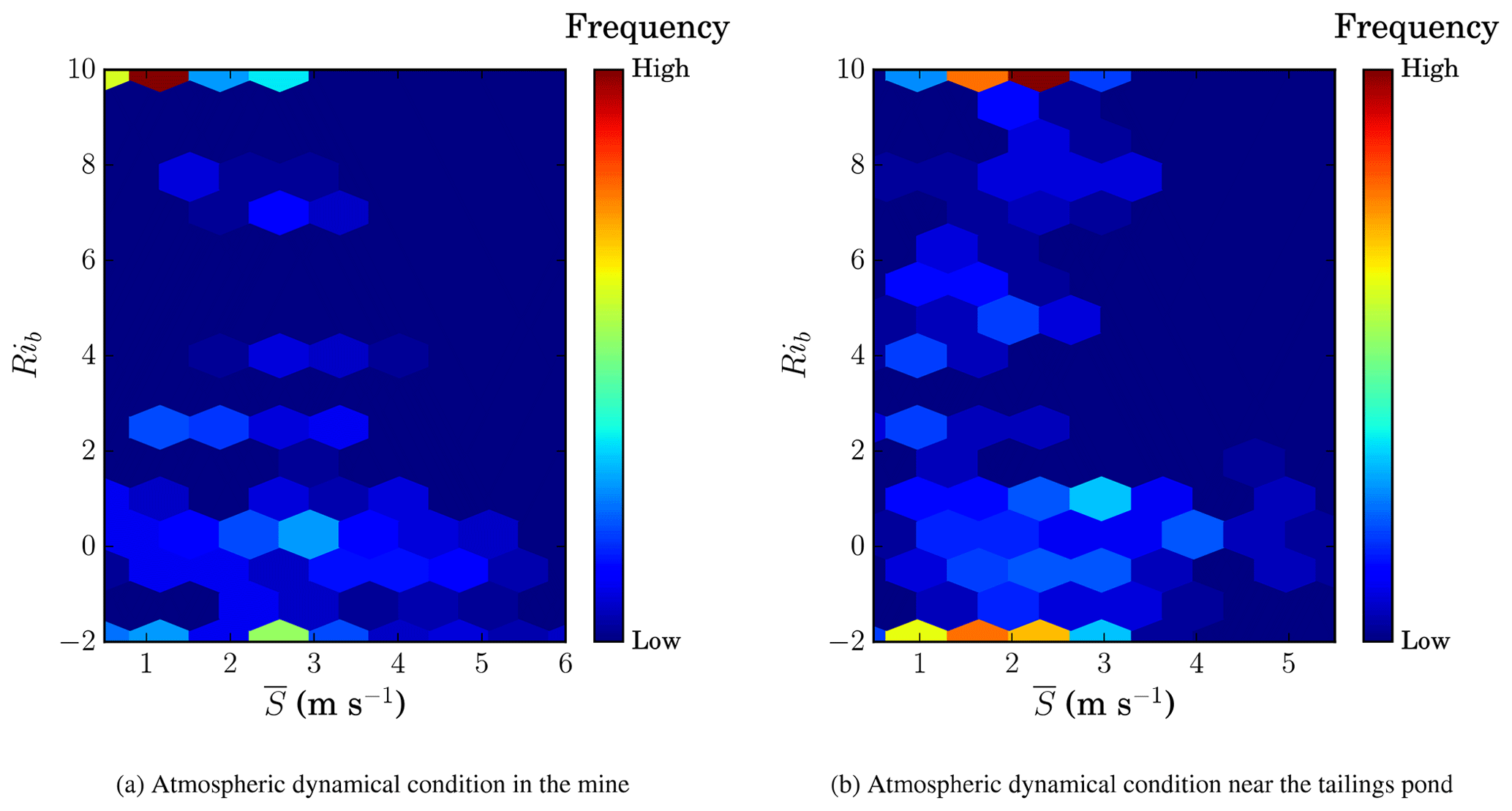
Figure 14 Frequency plots of atmospheric dynamical condition as a function of bulk Richardson number Ri_b and mean wind speed $\stackrel{\mathrm{‾}}{S}$ in the mine (a) and near the tailings pond (b).

5 Conclusions and future work

The vertical structure of the ABL in an orographically complex terrain, such as a mine, can be complicated. TAB has provided an acceptable platform for the meteorological measurements inside the surface layer within ABL and atmospheric dynamical condition over a complex terrain of a mining facility. The field campaign took place in May 2018 in northern Canada. In the surface layer, most atmospheric transport mechanisms are highly influenced by the terrain complexity. TAB measured the microclimate in the complex terrain by quantifying mean and turbulence statistics of the atmospheric meteorological variables. This was achieved by sensing the components of the wind velocity vector, temperature, relative humidity, and pressure. The calculated variables included mean horizontal wind speed, turbulence kinetic energy, friction velocity, Obukhov length, vertical kinematic sensible heat flux, variance of potential temperature, and variance of vertical wind velocity. TAB further determined the atmospheric dynamical condition by specifying the combination of the thermal stability state (bulk Richardson number) and mean horizontal wind speed.

TAB observed that the wind speed, turbulence kinetic energy, and friction velocity exhibit a significant diurnal variation, indicating calm conditions during nighttime and early mornings, when the atmospheric diffusion coefficient is low, and gusty conditions in the mid-afternoons, when the atmospheric diffusion coefficient is high. TAB also revealed the vertical structure of the atmosphere near the surface for most meteorological variables. The highest turbulence kinetic energies occurred in the lowest 100 m above the surface, albeit for small fluctuation timescales and length scales probed. Experiments provided evidence for the variation of thermal stability and wind speed as a function of diurnal time. The atmosphere spent a considerable amount of time under near-neutral and stable conditions, with implications on atmospheric diffusion coefficient and emission fluxes of atmospheric constituents released near the surface. The experiments specifically observed differences in the microclimate in the mine pit in comparison to that near the tailings pond. The overall pattern of diurnal variation was found to be similar for both the mine and the tailings pond, but subtle meteorological differences were observed. The mean wind speed, turbulence kinetic energy, and friction velocity were comparatively lower in the mine than near the tailings pond under thermally stable conditions, suggesting that the mine boundary layer may have been isolated from the boundary layer above grade. In addition, more positive vertical kinematic sensible heat flux and potential temperature variance were observed in the mine in various diurnal times in comparison to the areas near the tailings pond. This was likely due to terrain complexity and anthropogenic activities in the mine.

A particular challenge in operating the TAB system is the proper choice of sampling time. On the one hand, short sampling times impose inherent errors in mean and turbulence statistics predictions while enabling high-resolution vertical measurements. On the other hand, long sampling times impose less inherent errors in mean and turbulence statistics predictions but they only enable low vertical resolution measurements. Another drawback of TAB system is that it is not autonomous, so it requires intensive operator effort to fly it. Future development requires advanced techniques for autonomous control of TAB.

Overall, TAB offers a simple and cost-effective platform for microclimate measurements within the atmospheric surface layer. The light high-frequency weather sensor on board enables measurement of mean and turbulence statistics of the atmospheric meteorological variables. This configuration allows a wide spatiotemporal coverage compared to fixed flux towers. TAB can potentially provide meteorological data as boundary conditions or validation datasets for developing high-resolution computational fluid dynamics and other mesoscale models that attempt simulating meteorological processes and emission fluxes from large complex terrains of mining and other similar facilities.