the Creative Commons Attribution 4.0 License.
the Creative Commons Attribution 4.0 License.
 | 07 Oct 2020
A global geographic grid system for visualizing bathymetry
Colin Ware
Larry Mayer
Paul Johnson
Martin Jakobsson
Vicki Ferrini
A global geographic grid system (Global GGS) is here introduced to support the display of gridded bathymetric data at whatever resolution is available in a visually seamless manner. The Global GGS combines a quadtree metagrid hierarchy with a system of compatible data grids. Metagrid nodes define the boundaries of data grids. Data grids are regular grids of depth values, coarse grids are used to represent sparse data and finer grids are used to represent high-resolution data. Both metagrids and data grids are defined in geographic coordinates to allow broad compatibility with the widest range of geospatial software packages. An important goal of the Global GGS is to support the meshing of adjacent tiles with different resolutions so as to create a seamless surface. This is accomplished by ensuring that abutting data grids either match exactly with respect to their grid-cell size or only differ by powers of 2. The oversampling of geographic data grids, which occurs towards the poles due to the convergence of meridians, is addressed by reducing the number of columns (longitude sampling) by powers of 2 at appropriate lines of latitude. In addition to the specification of the Global GGS, this paper describes a proof-of-concept implementation and some possible variants.
- Article
(4878 KB) - Full-text XML
- BibTeX
- EndNote


It is safe to say that geographic coordinates are by far the most widely used method for specifying locations on the Earth's surface. They are also used commonly to specify regular grids of height values sometimes called digital terrain models (DTMs) or digital elevation models (DEMs) (Li, 2004). A great advantage of these is compact storage, because with a geographic grid, individual grid cell locations need not be stored; instead it is only necessary to specify a bounding box in geographic coordinates, together with the number of rows and columns. Given equal spacing, the location of an individual grid point can be easily computed. Unfortunately, when portrayed on a sphere, grids based on geographic coordinates suffer from problems at the geographic poles due to convergence of meridional lines. This results in oversampling in the zonal direction (along lines of latitude). The global geographic grid system (Global GGS) proposed here is designed to retain the advantages of geographic coordinates while minimizing the problems of oversampling at the poles.
The term geographic coordinates commonly refers to the use of latitude, longitude and elevation to specify a location on Earth. The concept has a very long history, dating to Eratosthenes of Cyrene in the third-century BCE (McPhail, 2011). The use of degrees to specify angle is similarly ancient, dating to the ancient Babylonians. The International Meridian Conference of 1884 set the 0 longitude meridian through the Greenwich Observatory in England and standardized the system that is used today.
The motivation for the gridding system described here comes from the Nippon Foundation-GEBCO-Seabed 2030 project. Seabed 2030 is an initiative to map the world's oceans to a set of specified resolutions by the year 2030 (https://seabed2030.gebco.net/, last access: 28 April 2020). Four depth bands are defined to be mapped at different resolutions: depths 0–1500 m at 100 m spatial resolution; depths 1500–3000 m at 200 m resolution; depths 3000–5750 at 400 m resolution and 5750–11 000 m at 800 m resolution (Mayer et al., 2018). The most recent gridded bathymetry covering all of the world's oceans is the GEBCO 2020 grid produced by the Seabed 2030 project (GEBCO Compilation Group, 2020). This grid is based on a depth database which covers 19 % of the world's oceans with some sort of depth measurement, primarily from single and multibeam sonars, calculated at the above-specified resolutions. However, it should be noted that the GEBCO 2020 grid itself is a regular geographic grid with a cell size of 15 arcsec.
1.1 Seafloor mapping
Most of what we know about the 71 % of Earth's surface that is covered by ocean waters has come through the mapping of the seafloor, yet only approximately 19 % of the depths have been directly measured (GEBCO Compilation Group, 2020). In recent years, multibeam echo sounders have been developed that have the ability to produce continuous high-resolution coverage over relatively wide swaths (typically 4–6 times the water depth) (Theberge, 1989; Wölfl et al., 2019). This evolution of ocean mapping technology has revolutionized our ability to produce bathymetric models and visualize seafloor bathymetry leading to much greater understanding of a range of Earth and ocean processes including insights into the tectonic evolution of the Earth, tsunamis, landslides and other marine geohazards, and a range of sedimentary processes. With the development of multibeam sonar technology has come a commensurate evolution in positioning technology (GPS and GLONASS) that has allowed the measurement of the bathymetry of the seafloor in a precise framework of geographic coordinates (Kumar and Moore, 2002).
But, as described above, to date, only a small percentage of sonar mapping data is available to produce updated bathymetric maps of the ocean floor (GEBCO Compilation Group, 2020). Beyond the sonar coverage, for most of the oceans there are virtually no direct bathymetric measurements. Instead, what is shown on global maps is predicted bathymetry derived from satellite measurements of ocean surface height indicating underlying bathymetry through gravity anomalies (Smith and Sandwell, 1997; Becker et al., 2009; Olson et al., 2014); predictions are constrained by directed measurements where they exist. Although predicted bathymetry is published in a global compilation at 15 arcsec resolution (approx. 463 m) (Tozer et al., 2019), the minimum size of features that can be resolved is actually much larger than this, because it is limited by the footprint of the satellite sensors and other environmental factors such as wind and wave effects (Smith et al., 2005). Typically, features smaller than 5–15 km horizontally cannot be resolved from predicted bathymetry alone.
The distribution of the Seabed 2030 resolution reflects a conservative view of the resolving ability of a modern multibeam sonar system deployed from a surface vessel operating in each of the water depth ranges (Mayer et al., 2018). Therefore, where only predicted bathymetry is available it can be stored and displayed at a lower resolution. Because of these requirements a system is needed to show data at varying resolutions, higher resolutions for shallower regions, where data exist, lower resolutions for deeper regions that have been mapped, and still lower resolutions where only predicted bathymetry exists.
The Global GGS tiling approach described herein is designed to meet the specific needs of the Seabed 2030 project though it can also have broader applications beyond. It is designed for simplicity in disseminating multi-resolution grids as specified by that project. It is also intended to support the purpose of computer graphics rendering. It is a pragmatic solution offering the advantages of regularly gridded data files for computer graphics and ease of resampling. It also offers compact file storage and the definition of all files as rectangles defined in geographic coordinates. It provides a nested hierarchy supporting data at any resolution; as such it should have uses for other projects involving the visualization of bathymetric or other geospatial gridded data beyond the specific requirements of Seabed 2030.
1.2 Existing grid systems
Three alternatives to the proposed Global GGS system are in common use for global bathymetry data: the geodesic-based hexagonal tiling developed by Sahr et al. (2003), the Mercator projection based system of Ryan et al. (2009), and the GEBCO geographic tiling system (Weatherall et al., 2015). There are also gridding schemes designed specifically for the computer graphics rendering of large gridded terrains.
The hexagonal tiling of Sahr et al. (2003) is an elegant system of overlapping hexagonal grids. Because the cells have approximately equal area, it is favored by flow modelers. However, it is more complex to implement and less space efficient in terms of storage since each point requires latitude–longitude and depth values. Moreover, resampling from fine meshes to coarser meshes is complex because tiles are not strictly nested at different resolutions.
The GMRT system of Ryan et al. (2009) is, in some ways, similar to Global GGS. It consists of a simple quadtree subdivision of the entire globe based on a Mercator projection. It differs from Global GGS in that it accommodates global coverage by maintaining three parallel tile sets – Mercator, south polar and north polar. For the projected system, it keeps a constant number of columns but varies the number of rows with latitude and, at a given level of binary subdivision, data grids increase in resolution with distance from the Equator. GMRT makes it simple to mesh data at a given resolution within one of the projections.
The GEBCO 2020 grid is a geographic system providing global bathymetry in geographic coordinates in a single grid at 15 arcsec resolution. It is not a hierarchical system, and because the grid is constant in geographic coordinates, the spatial density of samples becomes increasingly asymmetric approaching the poles where sample spacing along lines of latitude becomes much greater than sample spacing along lines of longitude.
Hierarchical meshes and grids have been extensively used in computer graphics applications for rendering both terrains and objects. Quadtrees in particular have been used for terrains. In most examples, the goal of a quadtree rendering is for run-time rendering of perspective views so as to render fewer polygons for more distant parts of the terrain. With hierarchical block representations (Pajarola and Gobbetti, 2007; Schneider and Westermann, 2006) fixed sized grids are used (257×257 in the case of Schneider and Westermann), and these are placed in a hierarchical structure. Regular grids can be rendered very efficiently by a modern computer graphics system so that even though these grids do not result in the minimum number of polygons overall, the gains in rendering efficiency outweigh the increase in polygon count. In addition, grids can be very compactly stored, since, as already mentioned it is not necessary to store the locations of each vertex or information about the triangular mesh.
The goals of storage for bathymetry data are significantly different than those for rendering surface terrains. In particular, our purpose is not primarily to support multi-resolution rendering, although that might be a side benefit, but to support the specific needs of bathymetric mapping that, due to limitations in data acquisition, are often constrained by data that vary in resolution with depth. The usual practice for block grids used in computer graphics (Schneider and Westermann, 2006) is for height values to be placed at grid vertices. In contrast, for bathymetric data it is more usual for depth values to be placed in the centers of grid cells. The value of the grid node is typically a statistical representation (mean, median, mode, etc.) of all of the soundings within a defined radius often with an inversely weighted contribution from surrounding cells. The two schemes are equivalent in terms of network topology, but there are important implications when it comes to sampling. Figure 1 illustrates this point. If points are defined at grid cell centers (a) averaging from a high resolution to a lower resolution is straightforward. The average of values within a 2×2 grid is the same as the average of the larger grid node one level up. This is not the case when heights (or depths) are placed at the vertices. Averaging the vertices shown in (b1) does not result in the vertices shown in (b2); rather it yields the vertices shown in (b3). In this case there are no points in common between grids at different resolutions, and some form of re-averaging is needed to achieve a grid hierarchy. There is little difference between the two schemes in terms of the complexity of stitching together adjacent grids since the meshes are topologically the same. Figure 1c and d show the triangular meshes required to stitch adjacent grids together in the two cases. The fill strip is narrower and skewed when depths are at the centers of grid cells.
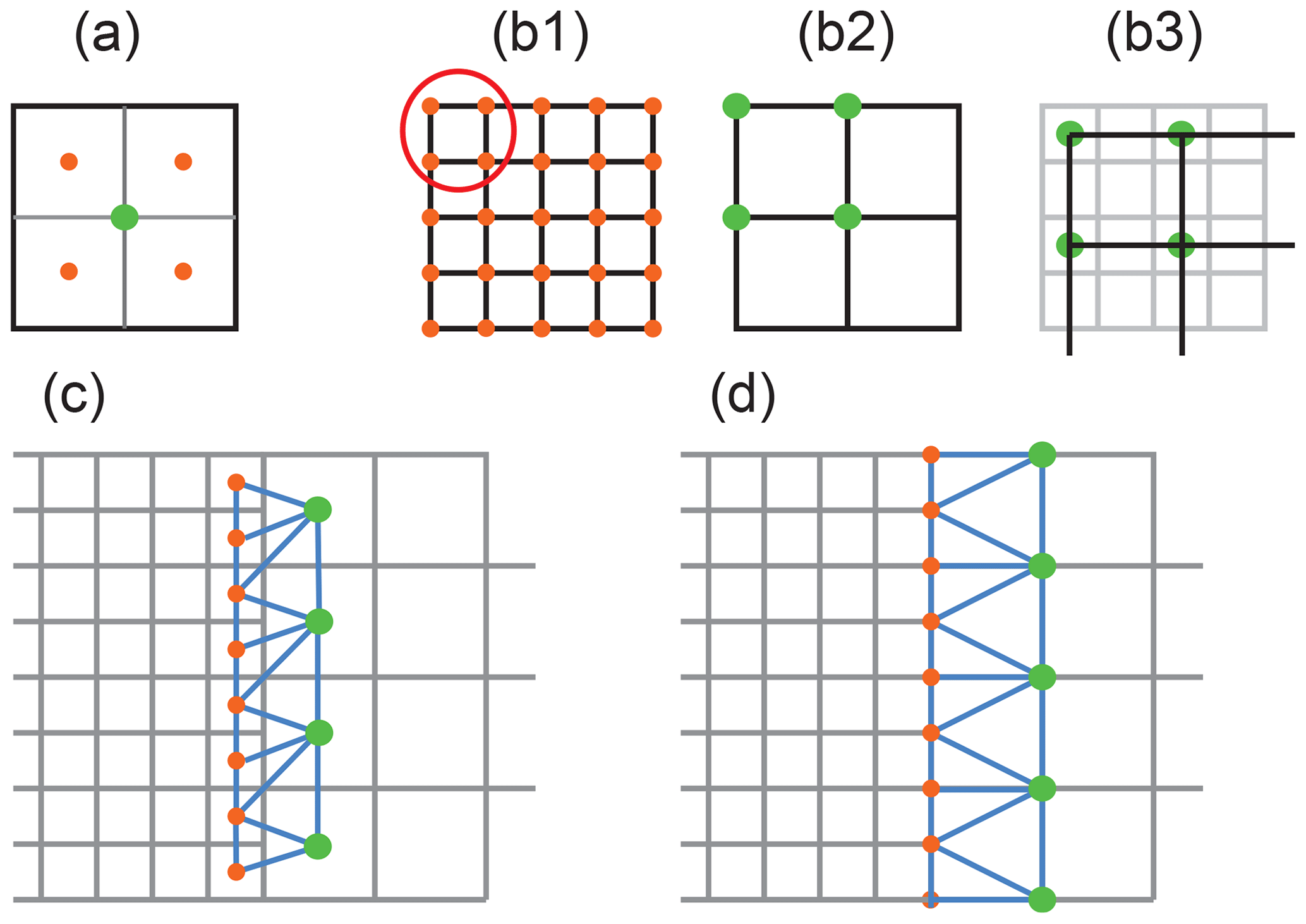
Figure 1(a) When depth values placed at the centers of cells are averaged to a lower resolution, the result is also at the center of a cell (green dot). (b) The averages of four vertex groups do not lie on vertices (b2) but at the centers of grid cells (b3), so there are no common vertices between grids at different scales. (c–d) Triangle strips linking adjacent grids are topologically the same for the two schemes.
The design goals for Global GGS were to create a hierarchical gridding system based on geographic coordinates and to mitigate the effects of variable sampling along lines of latitude, which occurs because of the convergence of meridians towards the geographic poles. It also makes it easy to tie together adjacent grids having different resolutions. In addition, for conceptual simplicity, it is desirable to have unit degrees as one of the possible grid sizes in the hierarchy. For this reason, a binary subdivision of the entire globe was rejected.
The Global GGS borrows from both GMRT and GEBCO; like GEBCO it is defined in geographic coordinates; like GMRT it incorporates a quadtree hierarchy enabling data of any resolution to be represented. Unlike GMRT, Global GGS uses a single scheme (and projection) to extend to the poles. Also, Global GGS avoids the extreme sampling asymmetries of GEBCO.

Figure 2(a) An example of a quadtree metagrid tree structure with a 2∘ subsection color coded to illustrate different data grid resolutions in meters. (Note that a 960×960 grid subtending 1∘ would have a grid cells size of 115.7 m.) (b) The same subsection is shown as a map. Numbers in the square areas illustrate grid sizes used to achieve different spatial resolutions.
The system supports differently sized data grids in a way that is independent of resolution. It is useful to have large tiles to represent large areas of the seafloor mapped at a constant resolution, but grids that are very large are slow to load and display and therefore difficult to handle in most interactive display systems. Smaller grids are space efficient for areas of the seafloor mapped at different resolutions, but numerous small grid tiles are also not efficient to render in computer graphics since large numbers of tiles must be managed. For this reason, Global GGS grids are constrained in both minimum and maximum size.
The Global GGS also supports the seamless meshing of low-latitude data with polar data sets. Often polar data sets use a different projection than the one used for data at lower latitudes creating difficulties in displaying data that cross the boundary. In the Global GGS, Arctic and sub-Arctic and Antarctic and sub-Antarctic data are supported essentially in the same way.
Global GGS combines a metagrid hierarchy with a system of compatible data grids. Metagrid nodes define the boundaries of data grids. Data grids are square grids of depth values, coarse grids are used to represent sparse data and finer grids are used to represent high-resolution data. Both metagrids and data grids are defined in geographic coordinates to allow broad compatibility with the widest range of geospatial software packages. An important goal of the Global GGS is to support the meshing of adjacent tiles with different resolutions so as to create a seamless surface. This is accomplished by ensuring that abutting data grids either match exactly or only differ by powers of 2. The oversampling of geographic data grids which occurs towards the poles is addressed by reducing the number of columns (zonal sampling) by powers of 2 at appropriate lines of latitude.
2.1 The metagrid structure
The metagrid is designed to have integer degrees as a basic unit with a quadtree structure starting at 8∘, which is the largest integer that both divides exactly into 360 and is a power of 2.
Figure 2 illustrates an example of a metagrid structure incorporating data grids of different sizes to achieve different resolutions in different regions; because this example is less than 8∘, the metagrid has a quadtree structure. Figure 3 illustrates the global metagrid. Up to 72∘ N or S, the metagrid consists of , , and ∘ cells as shown in Fig. 2, with a quadtree for cells of 8×8 and smaller as shown in Fig. 1; at 72∘ N or S, the metagrid becomes and at 80∘.
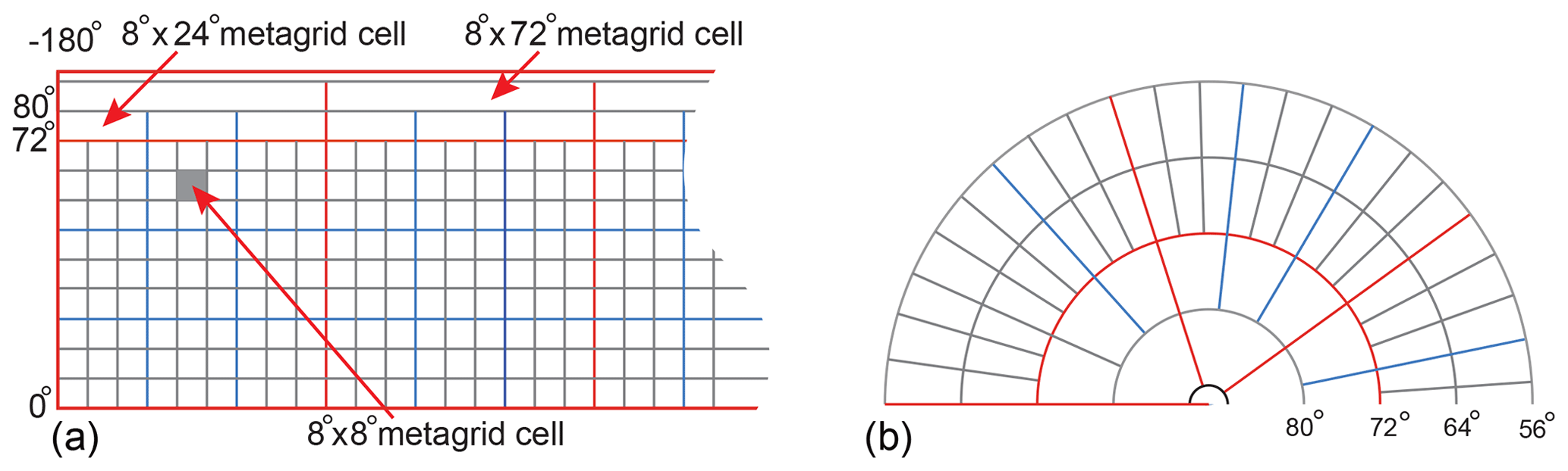
Figure 3(a) The metagrid is shown above the Equator. For cells 8×8 and smaller the structure is a quadtree. (b) A polar view of the metagrid showing wider metagrid cells north of 72∘.
2.2 Data grids below 60∘ N or S
Data grids have their row and column counts defined in powers of 2, and to support efficient tiling have both a minimum and a maximum allowable (row, column) size. Because both metagrids and data grids are defined by powers of 2 the system guarantees that abutting meshes only differ by powers of 2 in terms of resolution. This greatly simplifies the stitching of adjacent cells.
All data grid cells are defined in terms of a binary sequence of resolutions. This results in a set of fixed spacings in terms of both degrees of longitude and physical distances in a north–south direction. In the east–west direction, the width of cells varies by a maximum factor of 2 at a given level of binary subdivision. For example, at 60∘ N or S, lines of longitude have half the separation that they do at the Equator.
For metagrid cells with a southern boundary <60∘, allowed sequences of data-grid sizes are for example: 64×64, 128×128, 256×256, 512×512, 1024×1024 (possibly also 2048×2048), or 60×60, 120×120, 240×240, 480×480, 960×960 (possibly also 1920×1920).
The latter sequence is fully compatible with the GEBCO 2020 grid. Tying such grids together at the boundaries is straightforward and because they always differ by powers of 2. In addition, resampling of the grids (or averaging down) is also simple. The reason for not having larger grid sizes is that large files are slow to load and inefficient when a small area must be viewed. The reason for not having smaller grid sizes is that rendering many small grids has a high computational overhead. In general, small grids will be used to render small features with large depth ranges, whereas the larger grids will be used for larger areas of uniform depth; as processing power and graphics efficiency increases, the range of data-grid sizes can easily be scaled.
2.3 The Arctic and Antarctic
The basic principle of polar grid construction is that the number of data grid columns decreases by powers of 2 as distances between lines of longitude decrease by a factor of 2. This gridding concept is illustrated in Fig. 4 with grid cells greatly enlarged for clarity. The first such boundary is at 60∘ where lines of latitude have half the spacing that they do at the Equator [cos (60)=0.5]. The next is at (approx.) 75.5∘ where lines of longitude half again. The third transition is above 82.8∘ where data grids have one-eighth of the number of columns per degree relative to rows.
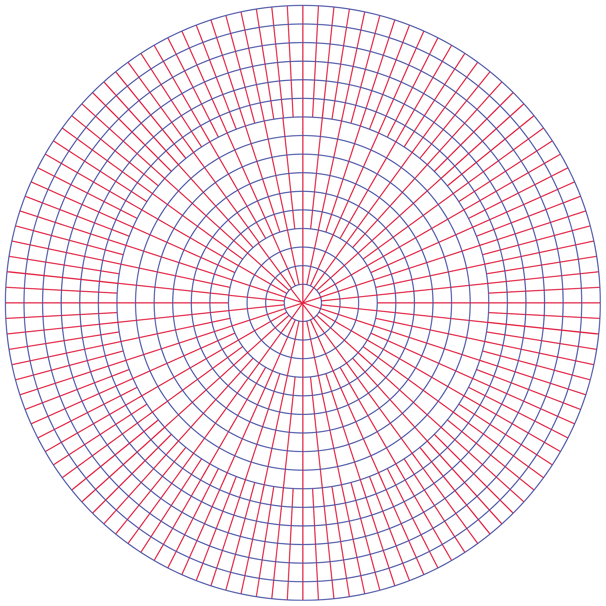
Figure 4For the polar regions the number of grid columns is reduced by two each time the spacing between lines of latitude is halved.
In addition to reducing the number of data grid columns on a per degree basis, metagrids become larger in the east–west direction as illustrated in Fig. 3. This is to avoid metagrids becoming very thin trapezoids, close to the pole. They become 24×8 at 72∘ N and 72×8 at 80∘ N. North of 88∘ is a single ∘ metagrid node.
To fit correctly within the 24×8 and 72×78 metagrid cells, data grids must be modified in such a way that they maintain the power of 2 ratio between abutting grids. Consider an example of a data grid based on a metagrid cell spanning 72–80∘ (latitude) and 0–24∘ (longitude). Were it not for the halving rule (north of 60) this data grid would contain 960 rows and 2880 columns, but because of the halving principle, above 60∘ it will have 960 rows and 1440 columns. Other allowable data grid sizes for this metagrid cell are 480×720, 240×360 and 120×180.
The wide high-latitude metagrid nodes form the roots of a quadtrees that subdivide in the same way as the 8×8 quadtrees at lower latitudes. So the child nodes of a ∘ metagrid node will be ∘, the grandchild nodes will be ∘ and so on.
In all cases the result is to create data grid cells where the east–west resolution is as good as, or better than, the north–south resolution.
2.4 Depths on vertices or centers?
Computer graphics renders polygons defined by vertices, and for this reason it is conceptually simpler if depth are defined at the vertices of data grids. If depths are defined at the centers of grid cells, small offsets must be computed relative to the metagrid frame and this adds complexity. Nevertheless, as discussed in the introduction, there is an advantage to having depths at the centers of data grid cells; it better supports both sampling and resampling from high-resolution to low-resolution grids. Global GGS can be implemented either with depths at grid centers or vertices. On balance, it is better for depths to be defined on grid centers.
2.5 Compatibility with GEBCO 2020 grid
The grid size sequence 60×60, 120×120, 240×240, 480×480, 960×960 is fully compatible with the GEBCO 2020 15 arcsec grid. This corresponds, for example, to a 960×960 grid within a 4∘ metagrid node (or 240×240 within a 1∘ metagrid node). More generally it is compatible with grid spacings in the series 30, 15, 7.5, 3.75… arcsec which correspond to 925.9, 462.9, 231.5, 115.7… m at the Equator.
The following sections describe a proof-of-concept implementation of the Global GGS. Source code is provided in a Bitbucket repository (https://bitbucket.org/ccomjhc/globalggs/, last access: 15 October 2019). The implementation was done in C and OpenGL and uses glut to provide a GUI for the test driver. Naturally, it could be implemented in any programming language, and there are many possible variations, some of which we discuss in a later section. In this description, we provide the main C classes and methods. Details relating to such things as shading and color-mapping are omitted since they are peripheral, but they are provided in the form of source code in the Supplement.
The implementation is driven by a latitude–longitude reference point. This causes the LoadData method to load a set of files within a specified distance from this point. On loading, all coordinates are converted to positions relative to the reference. The use of relative positions has the important benefit that coordinates can be stored as single, as opposed to double, precision floats substantially reducing the memory load.
3.1 The GGGS root class
The GGGS root class is an implementation of the top level grid illustrated in Fig. 3. The main data structure is a two-dimensional (24×45) array of pointers to metagrid nodes. The grid has a longitude range of (−180∘, 180∘). The latitude range of the array extends beyond the poles, from −96.0 to 96∘. This ensures a grid boundary at the Equator but means that the first and last rows only contain 2∘ of data. The nodes approaching the Equator have extended widths (, , ∘). However, these are implicit as illustrated in Fig. 5 and maintained by the accessor functions.
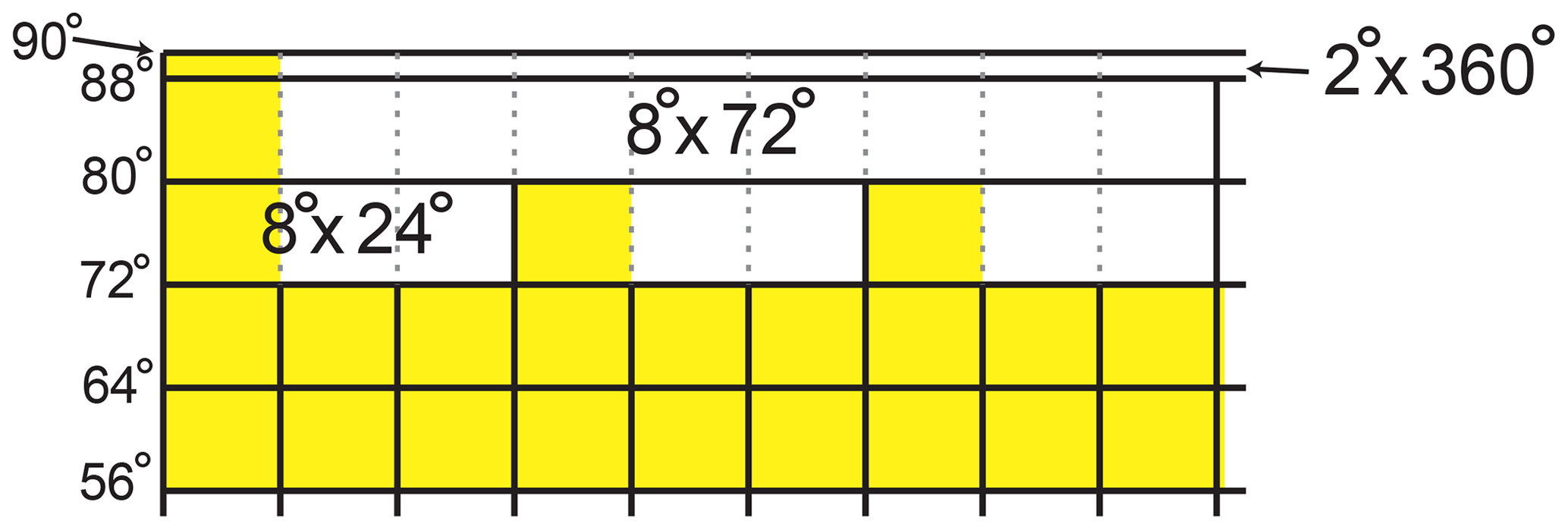
Figure 5The larger root nodes north and south of 72∘ are implicit. Only the nodes colored yellow contain pointers to metagrid subtrees.
The implementation relies on pre-prepared data grid files with grids that are computed as described in the first part of the document.
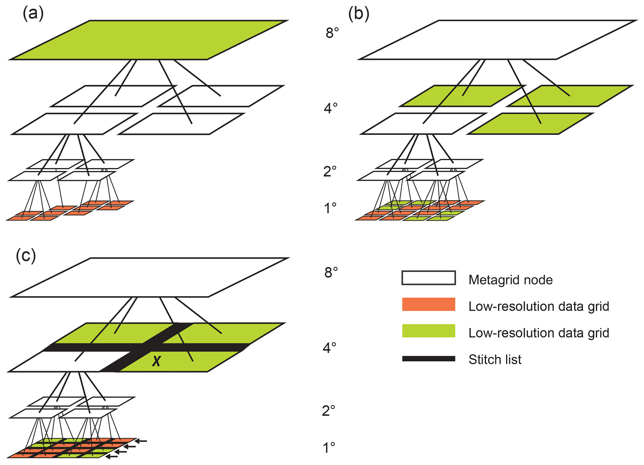
Figure 6Steps in the construction of a seamless mesh from multi-resolution files. (a) The structure after the data have been loaded. (b) The structure following pushdown. (c) Following stitchList construction.
There are three public methods in the GGGS root class: LoadData, draw and loadColorMaps.
LoadData (float lat, float long,
float width, float height)
The LoadData method takes in a latitude–longitude reference point as well as a width (in longitude degrees) and a height (in latitude degrees). Its main function is to sequence various operations carried out by the metaGridNode class. These are listed here then described in more detail in the descriptions of metaGridNode methods.
-
LoadData first instantiates a set of metaGridNode objects covering the specified ranges.
-
LoadData inserts the top level (or in polar regions: , , ∘) data files covering the specified range. For this implementation low-resolution data grids are required to exist for all top level metagrid nodes.
-
Within the boundaries of each metaGridNode the entire set of file names for 1×1 (or in polar regions: , , or ∘). nodes are constructed. Their existence is tested the filenames for those that exist are passed to the metaGridNode. An alternative approach would be to have a list of files available for insertion based on a pre-defined scene file. Figure 6a shows an example tree following data insertion.
-
For each top level metaGridNode the pushdown method is called. This recursively splits the top level metagrid node into parts to fill in around the detail nodes in the metaGridNode tree. Figure 6b shows an example tree following this operation.
-
For each top level node a linkSibs metagrid method is called. This recursively threads the tree, linking pointers between nodes at every level. At every level it is the parents responsibility to provide each child node with pointers to their siblings.
-
For each top level metaGridNode a walkBuildStrips(0 method is called. The purpose of this is to build stitchLists for every data grid node which will be displayed. A stitchList is an array of arrays containing the data points of the nodes adjoining the east, west, north and south edges of a displayable data node. stitchLists are needed to fill the strips between data grids with polygons. Figure 6c shows an example tree following this operation.
-
Special stitchLists are constructed for the boundaries at 72 and 80∘ if these boundaries lie within the specified latitude–longitude data ranges.
draw (bool lores)
The draw method calls the root metaGridNodes which then traverse the hierarchical metaGridNode trees and draws both the data grids and their associated stitchLists. The draw method has a single boolean parameter. If set to true rendering is done at lower resolution. This is useful for interactively changing the view of the data.
loadColorMaps()
The loadColorMaps method loads multiple colormaps so that attributes of the data sets can be color coded.
3.2 The metaGridNode class
metaGridNode implements the quadtree hierarchy, a signature feature of the Global GGS. Each metagrid node has four pointers to children which are also metaGridNodes. Each node also has pointers to sibling nodes to the east, west, north and south. The following sections describe the functions of the most important class methods.
bool insertChild (char *fname,
double focusLat, double focusLon,
int childC, int childR, int depth,
int Tdepth);
The insertChild method is passed a file name, the focus latitude–longitude coordinates, depth of insertion and the current depth within the metaGridNode tree. The childC and childR parameters tell it which (of four) children it is, relative to its parent.
insertChild builds the metaGridNode tree down to the level at which the data file should be inserted. Once that level is reached the bathyGrid method is given the responsibility of opening and loading the data file. Figure 7 shows an example which crosses the 80∘ boundary.
pushdown (int depth);
pushdown is a recursive method which takes any node that both contains a bathyGrid and has children. It passes down a pointer to the bathyGrid to all of its child nodes using the insertDtmQuadrant method. These child nodes extract the bathyGridNode quadrant corresponding to their geographic extent and copy the data into a new bathyGrid node. This is recursively repeated to the lowest level in the hierarchy. The purposes is to fill in around high-resolution nodes which have been inserted. Figure 6b illustrates the result as a tree diagrams. Figure 8 gives an example.
insertDtmQuadrant (bathyGrid *ddtm,
int child)
insertDtmQuadrant is passed an instance of a bathyGrid, together with information about which (of four) children it is, relative to its parent. It uses this information to create a new bathyGrid using the appropriate quadrant of the bathyGrid.
dtmQuadrantMerge (bathyGrid *ddtm,
int child)
For this implementation there is an additional dtmQuadrantMerge function with is called when the traversal reaches a leaf node. The 1∘ data grids in this application only contain valid bathymetry, where multibeam surveying has been done, otherwise they are empty. dtmQuadrantMerge is used where leaf nodes contain multibeam bathymetry. In these cases, the low-resolution bathyGrid is interpolated to fill the missing values as illustrated in Fig. 8.
linkSibs (int mg8Lat, metaGridNode *sE,
metaGridNode *sW, metaGridNode *sN,
metaGridNode *sS);
LinkSibs is a recursive method that walks the tree connecting sibling pointers to adjacent metaGridNodes at each level. It is the parents responsibility to give each child pointers to its siblings.
buildStitchLists()
buildStitchLists is responsible for building a data structure required to fill the gaps between adjacent nodes with strips of polygons. The method creates and populates a data structure which is a list of lists. Stitch lists are only required where larger nodes are adjacent to a set of smaller nodes along one of the edges and they are only built for leaf nodes (that have no children). An example is given in Fig. 6 where the node marked with an X will have a stitch list along it's western edge containing the data points from the extern boundaries of the four nodes indicated by arrows.
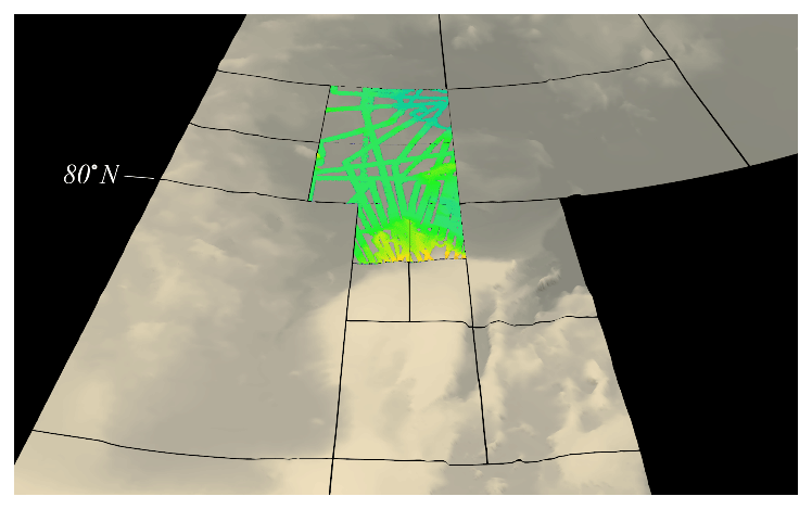
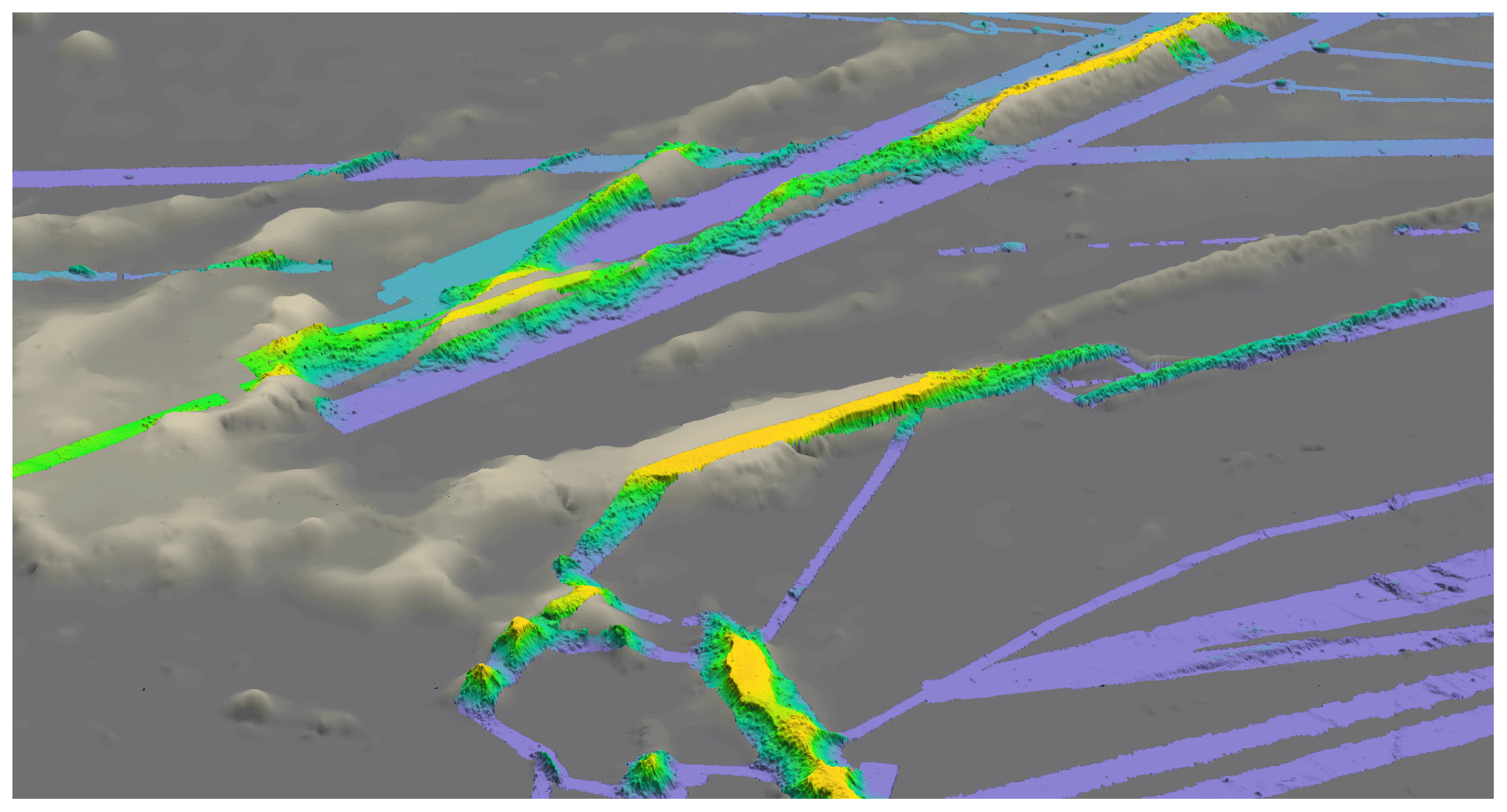
Figure 8In this example, a low-resolution grid has been used to fill in around a high-resolution multibeam data. Two colormaps are used with highly saturated colors being used to highlight multibeam data.
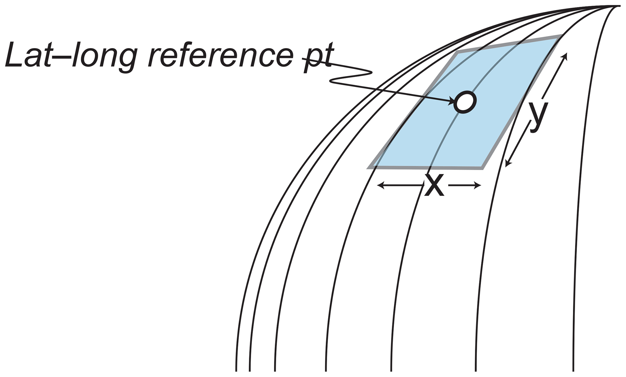
Figure 9Bathymetric values are represented relative to a tangent plan with an orthographic projection of latitude–longitude positions.
For leaf nodes, buildStitchLists checks the east, west, north and south neighbors. If they exist, then a stitch list is constructed, by asking that neighbor to fill in the data points for the appropriate edge. If a neighbor is not a leaf node this involves recursively traversing the neighbor's subtree. For example, building a stitch list for the west edge of node X in Fig. 6c involves obtaining a list of the data grid values along the east edges of the leaf nodes indicated by arrows.
3.3 The bathyGrid class
bathyGrid nodes load and store load data from bathymetry files, computes surface normals, and renders the data. For this implementation latitude–longitude coordinates are transformed by rotations into a planar orthographic projection centered on the focus coordinates (Fig. 9). Because all coordinates are stored as offsets from the focus coordinates and this means that single precision floating point numbers can be used internally. On loading a data grid, latitude–longitude coordinates are constructed for the centers of all grid points based on the lower left coordinate of a data grid, the grid size and the number of rows and columns.
computeXYfromLatLon (double focLat,
float focLon, float rLat, bool print)
These coordinates are transformed to x, y coordinates on a plane tangential to the surface at the reference point. This is achieved by rotating the absolute latitude and relative longitude values about an axis through the Equator. This yields x, y coordinates for each of the DEM points as illustrated in Fig. 9.
Perhaps the most important practical implication of Global GGS is that it constrains a set of dissemination grids. In order for the system to be efficiently implemented these must be defined at a series of resolutions given by binary subdivisions of degrees as prescribed. In the ideal situation, data grids will be derived directly from primary data sources such as bathymetric measurements from multibeam mapping systems. However, in many cases it is inevitable that resampling from existing grids will be necessary.
Although Global GGS prescribes the grid spacings, it is agnostic as to the format of data grid files. In the implementation provided in supplementary material, bathymetry is encoded compactly using png files, but GeoTIFFs, NetCDF files or any other gridded format could serve the purpose. Also, there are other variants in file format which could be implemented within the Global GGS concept. For example, adding additional rows and columns to grid boundaries which duplicate the boundaries of adjacent grids, could facilitate the rendering of seamless tiling where a single resolution is involved.
One of the less than desirable qualities of Global GGS is non-square grid cells. In Global GGS data grids can have variable aspect ratios between 1.0 and 2.0 depending on latitude. However, where the aspect ratios are higher, this represents an oversampling in terms of longitude, never an under sampling. A simple modification could be used to ensure that the aspect ratio never exceeds the square root of 2 (1.4142). This can be achieved by changing the latitudes at which the number of columns is decreased. For example, instead of the first such transition occurring at 60∘. of latitude it would occur at 45∘. But this modification would also have a cost in that sometimes longitude would be oversampled with respect to latitude and sometimes the converse.
There are many alternative ways in which Global GGS could be implemented either as a desktop or web-based application. The specific implementation given here is provided only as a working example. Some aspects of it are more general than others. The way the tree is built, as files are inserted, would be a necessary part of any implementation. The pushdown function is also needed to fill around high-resolution data with lower-resolution data. Some form of threading between adjacent nodes will be needed in order to provide links necessary to create seamless polygon meshes at the boundaries between data grids, especially those having different resolutions. Other aspects of the implementation are open to many alternatives. The specific way that the boundary links are constructed using stitchLists is just one possibility.
For many applications the implementation of scene files would be a useful enhancement. These could specify an assemblage of data grid files and attribute files, together with rendering attributes such as colormaps, viewpoint, height exaggeration and illumination.
As discussed in the introduction, the use of small tiles has the advantage that they can be loaded rapidly for interactive applications especially over the internet. Small grids are also beneficial where the resolution at which the seafloor has been mapped is highly variable, as is often the case for bathymetric data, especially where the data has been acquired to support science rather than standardized surveys conducted by hydrographic agencies. Smaller files lead to efficient rendering by reducing the number of polygons for terrains where only isolated areas have high-resolution data. But there are circumstances where larger tiles may be more beneficial, especially where larger areas with limited relief have been uniformly mapped. With some storage schemes rapid loading need not be compromised by large file sizes. For example, NetCDF files, allow for rapidly loading subsets of the data within a file without the whole file being read.
The original motivation for Global GGS came from the Seabed 2030 project and its need for multi-resolution grids which requires a method capable of handling multiple resolutions in a seamless mesh. However, different resolutions were also specified as a minimum requirement, meaning that higher resolutions could eventually be accepted and making it desirable to design a system that can support any resolution. Global GGS meets this requirement and can support the visualization of grids at any resolution. As such Global GGS may also prove to be an efficient approach to the representation of any single or multiresolution globally distributed three-dimensional geospatial data set.
Example code is available in a bit bucket repository https://bitbucket.org/ccomjhc/globalggs (Ware, 2019, last access: 15 October 2019). Note that the concepts in this paper are more general than those expressed in the code which represents a proof-of-concept implementation. There are many possible implementations of Global GGS and many useful variants.
A small amount of sample data is available in the same bit bucket repository https://bitbucket.org/ccomjhc/globalggs (Ware, 2019b, last access: 15 October 2019).
CW developed the original concept, wrote the code, did most of the writing. LM helped to refine the concept, provided advice on issues related to mapping. Wrote much of the introduction. PJ: Transformed data grids for prototype. Advised on mapping and GIS formats. MJ helped to clarify the concept. Advised with respect to Arctic data requirements. VF helped to refine the concept. Helped with data preparation and the transformation of GMRT (Mercator) data into the GGGS format.
The authors declare that they have no conflict of interest.
This work was supported by NOAA Grant NA15N0S400200 to the Center for Coastal and Ocean Mapping, UNH (Mayer PI and Ware Co-PI).
This research has been supported by the National Oceanic and Atmospheric Administration (grant no. NA15-NOS4000200).
This paper was edited by Fernando Nardi and reviewed by two anonymous referees.
Becker, J. J., Sandwell, D. T., Smith, W. H. F., Braud, J., Binder, B., Depner, J. L., Fabre, D., Factor, J., Ingalls, S., Kim, S. H., and Ladner, R.: Global bathymetry and elevation data at 30 arc seconds resolution: SRTM30_PLUS, Mar. Geod., 32, 355–371, 2009.
GEBCO Compilation Group: GEBCO 2020 Grid, edited by: The Nippon Foundation-GEBCO-Seabed 2030 project, https://doi.org/10.5285/a29c5465-b138-234d-e053-6c86abc040b9, 2020.
Kumar, S. and Moore, K. B., The Evolution of Global Positioning System (GPS) Technology, J. Sci. Educ. Technol., 11, 59–80, 2002.
Li, Z.: Digital Terrain Modeling: Principles and Methodology, 1st Edn., CRC Press, Boca Raton, 323 pp., 2004.
Mayer, L., Jakobsson, M., Allen, G., Dorschel, B., Falconer, R., Ferrini, V., Lamarche, G., Snaith, H., and Weatherall, P.: The Nippon Foundation – GEBCO seabed 2030 project: The quest to see the world's oceans completely mapped by 2030, Geosciences, 8, 10–27, 2018.
McPhail, C. K.: Reconstructing Eratosthenes' Map of the World: A Study in Source Analysis (Doctoral dissertation, University of Otago), 190 pp., 2011.
Olson, C. J., Becker, J. J., and Sandwell, D. T.: A new global bathymetry map at 15 arcsecond resolution for resolving seafloor fabric: SRTM15_PLUS, in: AGU Fall Meeting Abstracts, 2014.
Pajarola, R. and Gobbetti, E.: Survey of semi-regular multiresolution models for interactive terrain rendering, Visual Comput., 23, 583–605, 2007.
Ryan, W. B., Carbotte, S. M., Coplan, J. O., O'Hara, S., Melkonian, A., Arko, R., Weissel, R. A., Ferrini, V., Goodwillie, A., Nitsche, F., and Bonczkowski, J.: Global multi-resolution topography synthesis, Geochem. Geophy. Geosy., 10, 1–9, 2009.
Sahr, K., White, D., and Kimerling, A. J.: Geodesic discrete global grid systems, Cartogr. Geogr. Inf. Sc., 30, 121–134, 2003.
Schneider, J. and Westermann, R.: GPU-friendly high-quality terrain rendering, J. World Soc. Comput. Graphic., 14, 49–56, 2006.
Smith, W. H. F. and Sandwell, D. T.: Global seafloor topography from satellite altimetry and ship depth soundings, Science, 277, 1957–1962, 1997.
Smith, W. H. F., Sandwell, D. T., and Raney, R. K.: Bathymetry from satellite altimetry: present and future, Proceedings of OCEANS 2005 MTS/IEEE, 17–23 September 2005.
Theberge, A. E.: Sounding pole to sea beam, in Paper Presented at the 1989 ASPRS/ACSM Annual Convention Surveying and Cartography, Silver Spring, (MD, NOAA Central Library), 334–346, 1989.
Tozer, B., Sandwell, D. T., Smith, W. H. F., Olson, C., Beale, J. R., and Wessel, P.: Global bathymetry and topography at 15 arc seconds, SRTM15+, Accepted Earth and Space Science, 2019.
Ware, C.: Global Geographic Grid System: demonstration code, 2019, GitHub repostitory, availabe at: https://bitbucket.org/ccomjhc/globalggs, last access: 15 October 2019a.
Ware, C.: Global Geographic Grid System: example data, 2019, GitHub repostitory, available at: https://bitbucket.org/ccomjhc/globalggs, last access: 15 October 2019b.
Weatherall, P., Marks, K. M., Jakobsson, M., Schmitt, T., Tani, S., Arndt, J. E., Rovere, M., Chayes, D., Ferrini, V., and Wigley, R.: A new digital bathymetric model of the world's oceans, Earth Space Sci., 2, 331–345, 2015.
Wölfl, A.-C., Snaith, H., Amirebrahimi, S., Devey, C. W., Dorschel, B., Ferrini, V., Huvenne, V. A. I., Jakobsson, M., Jencks, J., Johnston, G., Lamarche, G., Mayer, L., Millar, D., Pedersen, T. H., Picard, K., Reitz, A., Schmitt, T., Visbeck, M., Weatherall, P., and Wigley, R.: Seafloor Mapping – The Challenge of a Truly Global Ocean Bathymetry, Front. Mar. Sci., 6, 1–9, 2019.