the Creative Commons Attribution 4.0 License.
the Creative Commons Attribution 4.0 License.
 | 16 Dec 2020
Mathematical foundation of Capon's method for planetary magnetic field analysis
Simon Toepfer
Yasuhito Narita
Daniel Heyner
Patrick Kolhey
Uwe Motschmann
Minimum variance distortionless projection, the so-called Capon method, serves as a powerful and robust data analysis tool when working on various kinds of ill-posed inverse problems. The method has not only successfully been applied to multipoint wave and turbulence studies in the context of space plasma physics, but it is also currently being considered as a technique to perform the multipole expansion of planetary magnetic fields from a limited data set, such as Mercury's magnetic field analysis. The practical application and limits of the Capon method are discussed in a rigorous fashion by formulating its linear algebraic derivation in view of planetary magnetic field studies. Furthermore, the optimization of Capon's method by making use of diagonal loading is considered.
- Article
(306 KB) - Full-text XML
- BibTeX
- EndNote


Nonlinear and adaptive filter techniques have a wide range of applications in geophysical and space science studies to find the most likely parameter set describing the measurement data or to decompose the data into a set of signals and noise. Above all, the minimum variance distortionless projection introduced by Capon (1969) (hereafter, Capon's method) has successfully been applied to multipoint data analyses for waves, turbulence fields and current sheets (Motschmann et al., 1996; Glassmeier et al., 2001; Narita et al., 2003, 2013; Contantinescu et al., 2006; Plaschke et al., 2008). The strength of Capon's method lies in the fact that the method performs a robust data fitting even when the spatial sampling or data amount is limited in the measurement (e.g., successfully applied to four-spacecraft data, Motschmann et al., 1996). Capon's method is currently being considered for planetary magnetic field studies in which the data (i.e., magnetic field samples) are more limited (e.g., data sampled on single orbits) and has recently been applied to simulated Mercury magnetic field data in view of the BepiColombo mission (Toepfer et al., 2020).
From a theoretical point of view there are several origins for the derivation of the method. The first derivation of Capon's method (Capon, 1969), constructed for the analysis of seismic waves, is based on the estimation of frequency–wavenumber spectra. Later on, this approach was reformulated in terms of matrix algebra (Motschmann et al., 1996). In light of mathematical statistics, Capon's estimator can be regarded as a special case of the maximum likelihood estimator (Narita, 2019). In this work the linear algebraic formulation of the method (Motschmann et al., 1996) with specific attention to magnetic field analysis is extended and the application of diagonal loading is discussed to improve the quality of data analysis with more justified applications and limits.
The analysis of planetary magnetic fields is of great interest and one of the main tasks in space science. Here we pay special attention to the analysis of Mercury's internal magnetic field, which is one of the primary goals of the BepiColombo mission (Benkhoff et al., 2010). The magnetometer onboard the Mercury Planetary Orbiter (MPO) (Glassmeier et al., 2010) measures the magnetic field vectors at N data points xi, along the orbit in the vicinity of Mercury. The magnetic fields around Mercury are considered to be a composition or superposition of internal fields generated by the dynamo process as well as crustal and induced fields, which are mainly dominated by dipole and quadrupole fields and external fields generated by the currents flowing in the magnetosphere. For Mercury the external fields contribute a significant amount to the total magnetic field within the magnetosphere (Anderson et al., 2011), and therefore a robust method is required for separating the internal fields from the total measured field. Yet, each component has to be properly modeled and parameterized when decomposing the field.
For example, when only data in current-free regions are analyzed, the planetary magnetic field is non-rotational and can be parameterized via the Gauss representation (Gauß, 1839). Within these current-free regions, the internal magnetic field can be expressed as the gradient of a scalar potential Φ, which can be expanded into a set of basis functions. Because of
the scalar potential Φ has to satisfy
where is the Laplacian. Choosing planetary centered coordinates with radius , azimuth angle and polar angle , the solution of Eq. (2) is given by spherical harmonics so that the potential results in
for the planetary dipole and quadrupole fields. Here, RM indicates the radius of Mercury and represents the Schmidt-normalized associated Legendre polynomials of degree l and order m. Within this series expansion a set of expansion coefficients and occurs, called internal Gauss coefficients. By constructing the Gauss coefficients in a vectorial fashion and defining the true coefficient vector as , the magnetic field vectors at every data point xi and the expansion coefficients are related via
where the terms of the series expansion are arranged in the matrix , called the shape matrix. The vector vi describes the parts that are not parameterized by the underlying model, e.g., the external parts, covering the range between the parameterized field and the measurement noise of the sensors, which is symbolized by the vector ni. The measurement noise is neither correlated with the parameterized part Hig nor with the non-parameterized part vi.
Summarizing the magnetic field measurements for all N data points into a vector , the field can be written as
where , and . G indicates the number of expansion coefficients.
Within Eq. (6) the magnetic field vector B and the shape matrix H, given by the underlying model, are known. The coefficient vector g is to be determined by data fitting. Since in most applications the number of known magnetic data points is much larger than the number of wanted expansion coefficients (G≪3N), H is a rectangular matrix in general. Furthermore, the non-parameterized parts of the field and the noise are unknown. Therefore, the direct inversion of Eq. (6) is impossible and g has to be estimated. In this case, Capon's method establishes a robust and useful tool to find the estimated solution for the expansion coefficients in Eq. (6).
Since the method does not require the orthogonality of the basis functions, it has a wider range of applications when decomposing the measured data into a set of superposed signals, especially when the number of data points is limited. For example, when the magnetic field data are measured on a dense grid in the vicinity of the planet, the Gauss coefficients can be estimated via integration of the data. But in the case of a limited data set those integrals cannot be evaluated.
The following derivation of Capon's method is based on the linear algebraic formulation (Motschmann et al., 1996), which was formerly applied to the analysis of plasma waves in the terrestrial magnetosphere. Now we are focusing on the analysis of planetary magnetic fields.
As illustrated in the previous section, the magnetic field bi measured at data point xi in the vicinity of Mercury and the wanted expansion coefficients g are related via
or in a compact form for all N data points
where the shape matrix H describes the underlying model.
For every data point xi the noise vector ni is assumed to be Gaussian with variance σn and zero mean so that 〈ni〉=0 and , where I is the identity matrix. The angular brackets indicate averaging over an ensemble, e.g., different samples, realizations or measurements. Therefore, holds and equivalently
since the model H and the true coefficient vector g are not affected by the averaging.
Because H is not always a square matrix but is in general a rectangular matrix with different sizes between rows and columns, the direct inversion of Eq. (9) is not guaranteed. Let us ignore for the moment the nonexistence of H−1 and write down the equation
Despite its simplicity it is obviously incorrect. As H−1 does not exist, let us look for another matrix w called the filter matrix, which follows the structure of this equation and in principle fulfills the solution of Eq. (9) with respect to g. Furthermore, the non-parameterized parts 〈v〉 are unknown, and therefore it is desirable to truncate these parts by the filter matrix. Capon's method is just the procedure to construct the filter matrix w and to calculate or, more precisely, to estimate g. To do so, some helpful quantities are introduced. In order to distinguish between the true coefficient vector g and the estimated solution, in the following Capon's estimator will be symbolized by gC.
For the inversion of Eq. (6) it is useful to rewrite the vectors B and gC in terms of a matrix representation. Thus, the data covariance matrix M and the coefficient matrix P are introduced as follows:
Here, Q indicates the number of measurements at each data point xi, for example the number of flybys at each data point, and the circle ∘ symbolizes the outer product, which is defined by
for any pair of vectors x∈ℝn, y∈ℝm. The dagger † indicates the Hermitian conjugate and the dot stands for the multiplication of the matrices and . Therefore, the diagonal of the matrix P contains the quadratic averaged components of the wanted estimator. It is important to note here that the covariance matrix M must be statistically averaged over several measurements. Otherwise the matrix is singular with a vanishing determinant (see Appendix A) and the further analysis cannot be achieved.
If the non-invertibility of the matrix Bα∘Bα is neglected, for every measurement α=1, …, Q an estimator for the true coefficient vector g can be determined so that
is valid. Thereby, each estimator deviates from the true coefficient vector by an error vector . Note that because of the non-invertibility of the matrix Bα∘Bα the single estimator cannot be calculated. Since the invertibility is solely given by the averaging over Q measurements, only the averaged estimator
with its related error
is available.
In contrast to the estimator, the true coefficient vector is a theoretical given vector that is not affected by the averaging (g≡〈g〉, Eq. 9). This property directly links the estimator to the true coefficient vector, which can be rewritten as
Averaging over Q measurements and using g≡〈g〉 results in
and analogously for the second-order moments
In the limit of vanishing errors 〈ε〉→0 and , Capon's estimator converges to the true coefficient vector:
and therefore
For the further evaluation of Eq. (6) the definition of the outer product (Eq. 13) is utilized. Matrix multiplication of Eq. (6) with its Hermitian adjoint and averaging yields
and therefore
assuming that n is Gaussian with variance σn and zero mean (〈n〉=0). Because H gC and 〈v〉 have the same dimension, the outer product commutates. By means of the limit 〈ε〉→0 in Eq. (21) the unknown matrix g∘g and the true coefficient vector g can be approximated by Capon's estimator, resulting in
Taking into account that and using the above defined abbreviations, Eq. (24) can be rewritten as
Since Eq. (25) cannot be directly solved for P, the goal is to find the best estimator gC for g so that is obtained as an approximate solution of Eq. (25). Therefore, a filter matrix w is constructed that separates the parameterized field from the noise by projecting the measured data onto the parameter space
and simultaneously truncates the non-parameterized parts, i.e.,
Applying the filter matrix to the average of the non-parameterized parts of the field in Eq. (6),
where the true coefficient vector has been replaced by Capon's estimator (Eq. 18) and taking into account that 〈n〉=0 leads to the distortionless constraint
This equation is one of the important constraints for the construction of the wanted filter matrix w, but it is not enough. Let us look for another criterion. The basic idea is that in Eq. (6) there may be contributions 〈v〉 in the data B that are not caused by the internal magnetic field, and thus these contributions are not modeled by H g. Although the filter matrix w is already designed to truncate these parts, i.e., , their contributions to the data are unknown, and therefore the parts that have to be truncated by w are unknown.
Referring to Eq. (26), the average output power, which is defined as the sum of the quadratic averaged components of the estimator, can be rewritten as (Pillai , 1989)
where tr 〈gC∘gC〉 is the trace of the matrix 〈gC∘gC〉.
Using Eq. (30), the coefficient matrix P can be expressed by the weight w and the data covariance M as
The amount of noise and the amount of the non-parametrized part are unknown. Thus, it is conservative and safe to assume that a large part of the data is influenced by the noise and the non-parameterized parts that have to be truncated by the matrix w and the underlying model keeps the minimal contribution to the data. This minimal contribution has to be extracted.
Therefore, the output power P=tr P has to be minimized with respect to w†, subject to the distortionless constraint or equivalently . Using the Lagrange multiplier method this minimization problem can be formulated as
where Λ represents the related Lagrange multipliers and the minimum is taken with respect to w. Since the components wij and of the matrix w and w†, respectively, are independent of each other, Eq. (32) can be expanded as
or equivalently
with related additional Lagrange multipliers Γ. Taking the derivatives with respect to wki and results in
yielding
and
resulting in
Multiplication of Eq. (36) with w from the right and multiplication of Eq. (38) with w† from the left considering the distortionless constraint delivers
and therefore
Because
is a convex function, Λ and Γ realize the minimal output power.
Due to the ensemble averaging the matrix M is invertible and M−1 exists. Multiplying Eq. (38) with and again considering the distortionless constraint yields
By means of Eq. (36) the filter matrix results in
and therefore Capon's estimator is given by
Regarding the expensive derivation, this compact formula for Capon's estimator is surprising.
The filter matrix w is the key parameter to distinguish between the parameterized and the non-parameterized parts of the field. Conferring to Eq. (25) the ratio of these parts defines the input signal–noise ratio (given by the data) as
The filter matrix is applied to the disturbed data for estimating the output power that is related to Capon's estimator. Thus, the output signal–noise ratio (resulting from the filtering) can be expressed as (Haykin, 2014; Van Trees, 2002)
since the filter fulfills the distortionless constraint and truncates the non-parameterized parts of the field, i.e., . The ratio of the output and the input signal–noise ratio is the so-called array gain (Van Trees, 2002),
which is controlled by tr(w†w), since H, P and v are given by the data and the underlying model.
The input signal–noise ratio is given by the data and the underlying model, and therefore in Eq. (47). In contrast to the input signal–noise ratio, the output signal–noise ratio depends on the filtering. When tr(w†w) is large, the output signal–noise ratio can decrease (SNRo→0), resulting in signal elimination, and thus the performance of Capon's estimator degrades. To prevent the signal elimination and to improve the robustness of Capon's estimator it is desirable to restrict tr(w†w) with an upper boundary (Van Trees, 2002), which can be expressed by the additional quadratic constraint
For reasons of mathematical aesthetics, the constant T0 is expressed as the trace of a matrix T. For example, one can choose
where G again indicates the number of wanted expansion coefficients and is the identity matrix so that
holds. Thus, Eq. (48) can be rewritten as
It should be noted that the matrix T can be chosen arbitrarily as long as it is independent of w and w†.
Referring to the previous section and considering the additional quadratic constraint, the filter matrix can be calculated by solving
with respect to w, where is the related additional Lagrange multiplier. Carrying out the same procedure as described in Sect. 3, the constrained minimizer is given by
The comparison of Eq. (43) with Eq. (53) shows that the quadratic constraint results in the addition of the constant value to the diagonal of the data covariance matrix M, which is known as diagonal loading (Van Trees, 2002). Consequently, the filter matrix is designed for a higher Gaussian background noise than is actually present (Van Trees, 2002).
In Fig. 1 tr(w†w) is displayed with respect to . For σd→0, tr(w†w) is large, resulting in a small output signal–noise ratio, which can cause signal elimination. For increasing values of σd, tr(w†w) decreases and for σd→∞ Capon's filter converges to the least square fit filter
or equivalently
which treats all data equally.
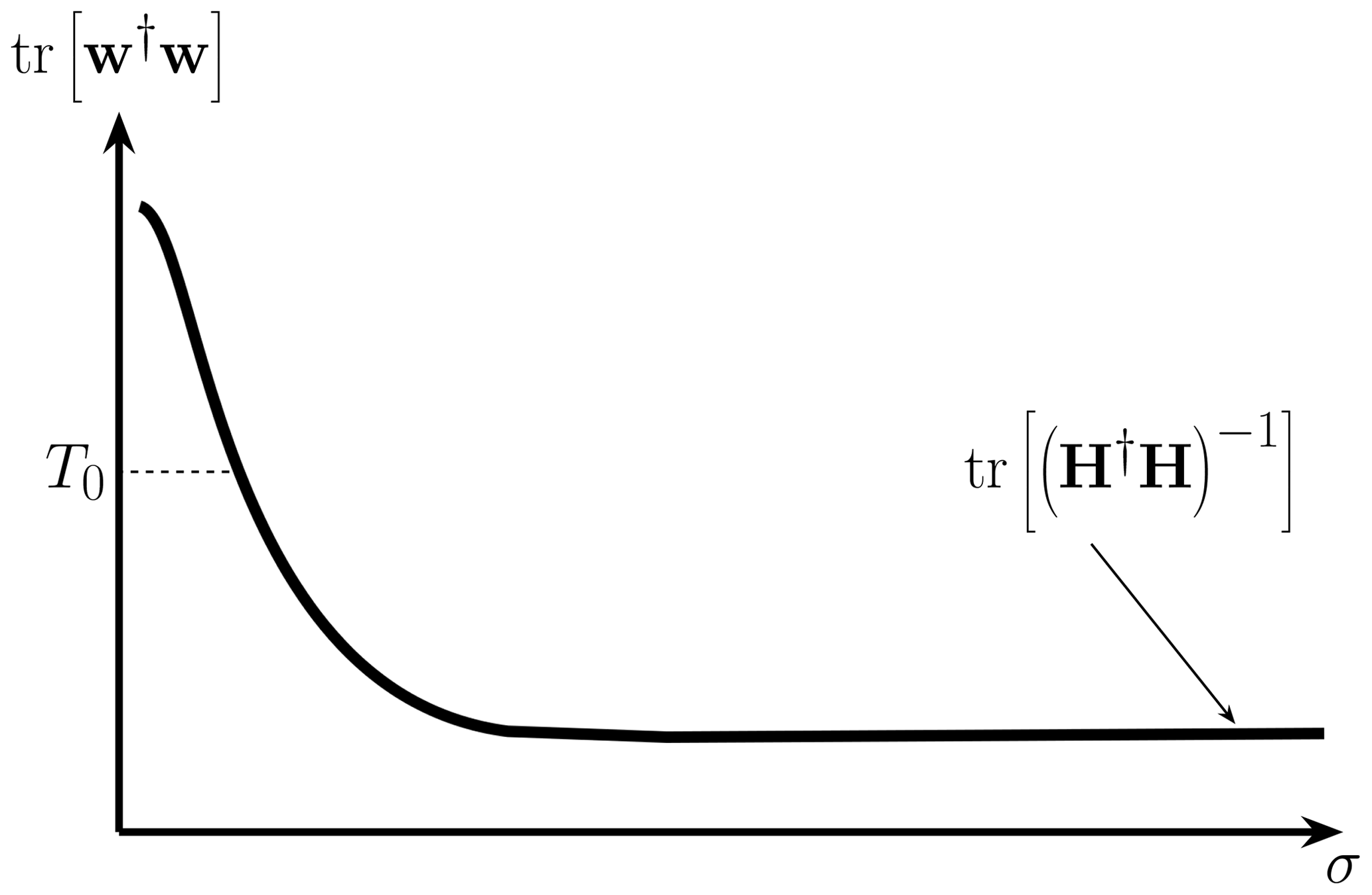
Figure 1Sketch of the trace of the filter matrix with respect to . For increasing values of the diagonal loading parameter σd the output signal–noise ratio increases and Capon's filter converges to the least square fit filter if the diagonal loading parameter is large.
Since tr(w†w) is a monotonically decreasing function, σd→∞ might be the best choice for the diagonal loading parameter. To check this expectation we have to take a look at the output power Pd for the synthetic increased noise, which can be estimated by replacing in Eq. (42), resulting in (Pajovic, 2019; Richmond et al., 2005)
Thus, Pd is an increasing function of σd. Since the output power has to be minimized one would expect that σd=0 is the best choice, which is in contradiction to the argumentation above. Therefore, the maximization of the array gain is not equivalent to the minimization of the output power (Van Trees, 2002). Since σd cannot be directly calculated within the minimization procedure (Eq. 52), it is not clear how to choose the optimal diagonal loading parameter σopt. that lies somewhere between those extrema.
In the literature there are several methods for determining the optimal diagonal loading parameter (Pajovic, 2019). In contrast to the analysis of waves, we favor measurements that are stationary up to the Gaussian noise for the analysis of planetary magnetic fields. Comparing the measurement times with planetary geology timescales, this assumption is surely valid for the internal magnetic field. For the external parts of the field this can be realized by choosing data sets of preferred situations, e.g., calm solar wind conditions. By virtue of the stationarity, the data covariance matrix contains only one nontrivial eigenvalue and for elsewhere (see Appendix B). Therefore, estimators for the diagonal loading parameter that are related to eigenvalues corresponding to interference and noise (Carlson, 1988) or estimators taking into account the standard deviation of the diagonal elements of the data covariance matrix, i.e., (Ma and Goh, 2003), cannot be applied. When simulated data are analyzed the deviation between Capon's estimator and the true coefficient vector, implemented in the simulation, is a useful metric for estimating the optimal diagonal loading parameter (Pajovic, 2019; Toepfer et al., 2020). But when the method is applied to real spacecraft data no true coefficient vector is available, and therefore another estimation method for the diagonal loading parameter that solely depends on the data and the underlying model is required.
The additional quadratic constraint (Eq. 48), resulting in diagonal loading, bounds the trace of the filter matrix that is the solution of the minimization procedure (Eq. 52). To prevent signal elimination, tr(w†w) and Pd have to be minimized simultaneously. Since tr(w†w) is decreasing for higher values of σd (see Fig. 1), Pd is an increasing function, and thus they act as competitors. At the optimal value σopt. the two competitors compromise, which can be understood as tr(w†w) reaches its minimal value under the constraint that Pd is minimal. Therefore, the diagonal loading of the data covariance matrix is equivalent to the Tikhonov regularization for ill-posed problems. The Tikhonov regularization improves the robustness of the least square fit problem,
with respect to g under the constraint of solutions g with minimal norm, i.e.,
where α is the corresponding Lagrange multiplier, which is also known as the regularization parameter (Tikhonov et al., 1995). In analogy to the Lagrange multiplier α, the optimal diagonal loading parameter can be estimated by the method of the L curve (Hiemstra et al., 2002). The L curve arises by plotting lg [tr(w†w)] versus for different values of σd and is displayed in Fig. 2. The optimal value σopt. is located in the vicinity of the L curve's knee, which is defined by the maximum curvature of the L curve (Hiemstra et al., 2002).
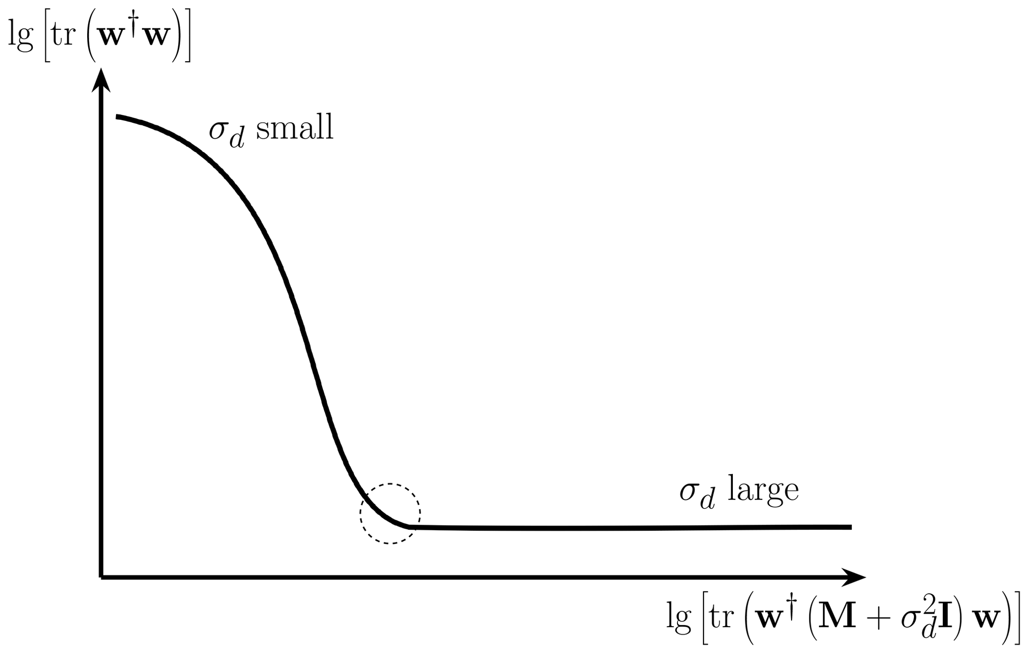
Figure 2Sketch of the L curve for estimating the optimal diagonal loading parameter σd. The optimal value is located in the vicinity of the L curve's knee (dashed circle).
When Capon's method is applied to the reconstruction of Mercury's internal magnetic field (Toepfer et al., 2020), several computationally burdensome matrix inversions are necessary to calculate the estimator (see Eq. 44)
Thus, for the practical application of Capon's method it is useful to rewrite the method in terms of the least square fit method.
Capon's estimator inherits the matrix operation structure of the least square fit estimator, which is given by Haykin (2014):
Substituting and in Eq. (60), the least square fit estimator may be converted into Capon's estimator.
The least square fit method minimizes the deviation between the disturbed measurements B and the underlying model H g, measured in the Euclidian norm , so that
Referring to the abovementioned substitutions, Capon's method can be interpreted as measuring the deviation in Eq. (61) in a different norm,
so that Capon's estimator is given by
Thus, Capon's method can be regarded as a special case of the least square fit method or more precisely of the weighted least square fit method, whereby the data and the model are measured and weighted with the inverse data covariance matrix. This property is useful for the practical application of Capon's method. In contrast to the computationally burdensome matrix inversions in Eq. (44), the usage of minimization algorithms, such as the gradient descent or conjugate gradient method, for solving Eq. (63) is more stable and computationally inexpensive.
To illustrate the mathematical foundations presented above, Capon's method is applied to simulated magnetic field data in order to reconstruct Mercury's internal magnetic field. As a proof of concept, the underlying model is restricted to the internal dipole and quadrupole contributions to the magnetic field as discussed in Sect. 2. Since simulated magnetic field data are analyzed, the special application to Mercury's magnetic field is of minor importance because the ideal solution is known from the simulation. If the method were tested against in situ measurement data, the application to the analysis of the Earth's magnetic field would be more suitable since the Earth's magnetic field is better known than Mercury's magnetic field.
For the reconstruction of Mercury's internal dipole and quadrupole field the internal Gauss coefficients and (Anderson et al., 2012; Wardinski et al., 2019), defining the nonvanishing components of the true coefficient vector g, are implemented in the hybrid code AIKEF (Müller et al., 2011), and the magnetic field data resulting from the plasma interaction of Mercury with the solar wind are simulated. The data are evaluated along selected parts of the prospective trajectories of the BepiColombo mission on the night side of Mercury within a distance of 0.2 RM up to 0.4 RM from Mercury's surface. Since simulated data are analyzed, the deviation between the true coefficient vector g and Capon's estimator gC can be used as a metric to verify the estimation of the optimal diagonal loading parameter by making use of the L-curve technique. The optimal diagonal loading parameter results in , which corresponds to the vicinity of the L curve's knee. The reconstructed Gauss coefficients for the internal dipole and quadrupole field are presented in Table 1.
Table 1Implemented and reconstructed Gauss coefficients for the internal dipole and quadrupole field.
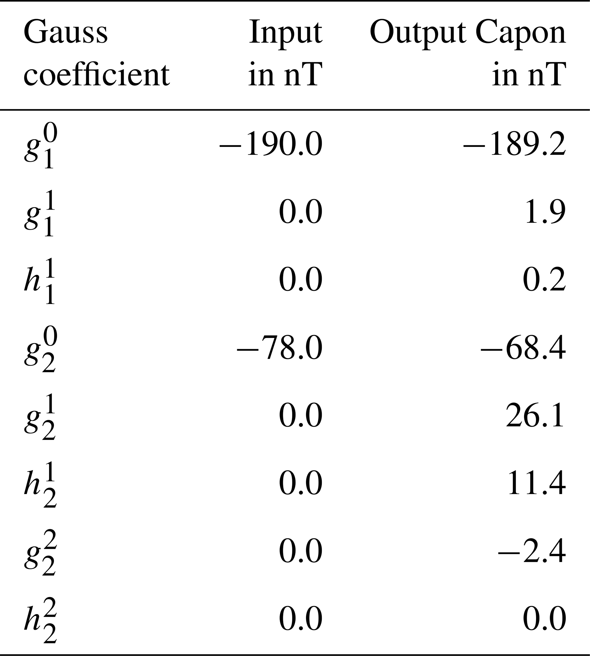
The deviation between Capon's estimator and the true coefficient vector results in 30.2 nT or 14.7 %, respectively, for the optimal diagonal loading parameter. When the magnetic field data are evaluated at an ensemble of data points at a distance of 0.2 RM from Mercury's surface this deviation is of the same order (Toepfer et al., 2020). Since the underlying model neglects the external parts and only the internal parts are considered, the coefficients and show large deviations from the implemented coefficients. Extending the underlying model by a parameterization of the external parts of the magnetic field improves Capon's estimator, especially when the magnetic field data are evaluated at some distance above Mercury's surface. In principle, one can also analyze the external field if some model is adopted.
Capon's method has been previously applied to the analysis of waves. Thus, the existing derivations treat the non-parameterized parts of the field v as Gaussian noise so that v and the measurement noise n are of the same character (Motschmann et al., 1996). Considering the analysis of planetary magnetic fields this assumption is indefensible. For example, the external parts of the field are systematic noise and cannot be modeled by a Gaussian distribution. When the non-parameterized parts are Gaussian, i.e., 〈v〉=0, the truncation of these parts by the filter matrix (see Eq. 27) is fulfilled trivially, which reduces the terms within the derivation and the estimation of the diagonal loading parameter. Therefore, the mathematical foundations presented above generalize the previous derivations of Capon's method and transist into the derivation presented by Motschmann et al. (1996) for the special case of 〈v〉=0.
As already mentioned in the Introduction (Sect. 1), Capon's method can be regarded from several mathematical perspectives. Within the derivation presented above, the output power P, which is defined as the trace of the coefficient (covariance) matrix, is minimized with respect to the filter matrix w, subject to the distortionless constraint . This procedure corresponds to the name minimum variance distortionless response estimator (MVDR), since P contains the variance of the model coefficients. Narita (2019) showed that Capon's estimator can also be derived by treating Capon's method as a special case of the maximum likelihood estimator by regarding the likelihood function as nearly Gaussian (particularly around the peak of the likelihood function). As discussed in Sect. 5, Capon's method can also be interpreted as a special case of the weighted least square fit. This illustrates that the several existing inversion methods for linear inverse problems are connected to each other and are not as different as they seem to be at first appearance.
Capon's method is a robust and useful tool for various kinds of ill-posed inverse problems, such as Mercury's planetary magnetic field analysis. The derivation of the method can be regarded from different mathematical perspectives. Here we revisited the linear algebraic matrix formulation of the method and extended the derivation for Mercury's magnetic field analysis. Capon's method becomes even more robust by incorporating the diagonal loading technique. Thereby, the construction of a filter matrix is vital to the derivation of Capon's estimator.
The trace of the filter matrix in particular determines the array gain, which is defined as the ratio of the output and the input signal–noise ratio. If the trace is large, the output signal–noise ratio can decrease, resulting in signal elimination, and thus the performance of Capon's estimator degrades. Bounding the trace of the filter matrix results in diagonal loading of the data covariance matrix, which improves the robustness of the method. The main problem of the diagonal loading technique is that in general it is not clear how to choose the optimal diagonal loading parameter. Since for the analysis of planetary magnetic fields we prefer measurements that are stationary up to the Gaussian noise, estimators for the diagonal loading parameter that are related to eigenvalues of the data covariance matrix corresponding to interference and noise cannot be applied. Making use of the L-curve technique enables a robust procedure for estimating the optimal diagonal loading parameter.
For the calculation of Capon's estimator several computationally burdensome matrix inversions are necessary. Interpretation of Capon's method as a special case of the least square fit method enables the usage of numerically more stable and fewer burden minimization algorithms, e.g., the gradient descent or conjugate gradient method, for calculating Capon's estimator.
It should be noted that the parameterization of Mercury's internal magnetic field via the Gauss representation, as mentioned in Sect. 2, is only one of several possibilities for modeling the magnetic field in the vicinity of Mercury. The underlying model can be expanded by other parameterizations, for example the Mie representation (toroidal–poloidal decomposition) or magnetospheric models, and Capon's method can be applied to estimate the related model coefficients. Besides the analysis of Mercury's internal magnetic field, the extension of the model also enables the reconstruction of current systems flowing in the magnetosphere. Concerning the BepiColombo mission this work establishes a mathematical basis for the application of Capon's method to analyze Mercury's internal magnetic field in a robust and manageable way.
The influence of the averaging on the determinant of the data covariance matrix M is exemplarily illustrated for the three-dimensional case. Thus, the magnetic field vector is given by
and therefore the outer product results in
with a vanishing determinant
Throughout the averaging of the data, the data covariance matrix results in
with a nonvanishing determinant
Thus, the inverse of M exists, whereas the outer product
B∘B is singular.
The data covariance matrix is defined as
This matrix is quadratic and especially diagonalizable. Thus, there is a matrix DM that is similar to the matrix M so that
where V is an orthogonal transformation, i.e., , and DM is a diagonal matrix, the diagonal elements of which are given by the eigenvalues of M. Inserting the definition of the matrix M delivers
since . To determine the diagonal form of the outer product, the two-dimensional case in which
is considered exemplarily. Thus,
and the characteristic polynomial results in
or equivalently
where β denotes the eigenvalue given by β=0 and . Therefore, in general the diagonal matrix of the outer product is given by
The noise matrix is already a diagonal matrix so that the diagonal form of M is given by
Thus, the data covariance matrix contains only one nontrivial eigenvalue and for .
The raw data supporting the conclusions of this article will be made available by the authors without undue reservation.
All authors contributed to the conception and design of the study; ST, YN and UM wrote the first draft of the paper; all authors contributed to paper revision as well as reading and approving the submitted version.
The authors declare that they have no conflict of interest.
The authors are grateful for stimulating discussions and helpful suggestions by Karl-Heinz Glassmeier and Alexander Schwenke.
We acknowledge support by the German Research Foundation and the Open Access Publication Funds of the Technische Universität Braunschweig. The work by Y. Narita is supported by the Austrian Space Applications Programme at the Austrian Research Promotion Agency under contract 865967. D. Heyner was supported by the German Ministerium für Wirtschaft und Energie and the German Zentrum für Luft- und Raumfahrt under contract 50 QW1501.
This paper was edited by Lev Eppelbaum and reviewed by two anonymous referees.
Anderson, B. J., Johnson, C. L., Korth, H., Purucker, M. E., Winslow, R. M., Slavin, J. A., Solomon, S. C., McNutt Jr., R. L., Raines, J. M., and Zurbuchen, T. H.: The global magnetic field of Mercury from MESSENGER orbital observations, Science, 333, 1859–1862, https://doi.org/10.1126/science.1211001, 2011. a
Anderson, B. J., Johnson, C., L., Korth, H., Winslow, R. M., Borovsky, J. E., Purucker, M. E., Slavin, J. A., Solomon, S. C., Zuber, M. T., and McNutt Jr., R. L.: Low-degree structure in Mercury's planetary magnetic field, J. Geophys. Res., 117, E00L12, https://doi.org/10.1029/2012JE004159, 2012. a
Benkhoff, J., van Casteren, J., Hayakawa, H., Fujimoto, M., Laakso, H., Novara, M., Ferri, P., Middleton, H. R., and Ziethe, R.: BepiColombo – Comprehensive exploration of Mercury: Mission overview and science goals, Planet. Space Sci., 85, 2–20, https://doi.org/10.1016/j.pss.2009.09.020, 2010. a
Capon, J.: High resolution frequency-wavenumber spectrum analysis, Proc. IEEE, 57, 1408–1418, https://doi.org/10.1109/PROC.1969.7278, 1969. a, b
Carlson, B. D.: Covariance matrix estimation errors and diagonal loading in adaptive arrays, IEEE Trans. Aerosp. Electron. Syst., 24, 397–401, https://doi.org/10.1109/7.7181, 1988. a
Constantinescu, O. D., Glassmeier, K.-H., Motschmann, U., Treumann, R. A., Fornaçon, K. -H., and Fränz, M.: Plasma wave source location using CLUSTER as a spherical wave telescope, J. Geophys. Res., 111, A09221, https://doi.org/10.1029/2005JA011550, 2006. a
Gauß, C. F.: Allgemeine Theorie des Erdmagnetismus: Resultate aus den Beobachtungen des magnetischen Vereins im Jahre 1838, edited by: Gauss, C. F. and Weber, W., Weidmannsche Buchhandlung, Leipzig, 1–57, 1839. a
Glassmeier, K.-H., Motschmann, U., Dunlop, M., Balogh, A., Acuña, M. H., Carr, C., Musmann, G., Fornaçon, K.-H., Schweda, K., Vogt, J., Georgescu, E., and Buchert, S.: Cluster as a wave telescope – first results from the fluxgate magnetometer, Ann. Geophys., 19, 1439–1447, https://doi.org/10.5194/angeo-19-1439-2001, 2001. a
Glassmeier, K.-H., Auster, H.-U., Heyner, D., Okrafka, K., Carr, C., Berghofer, G., Anderson, B. J., Balogh, A., Baumjohann, W., Cargill, P., Christensen, U., Delva, M., Dougherty, M., Fornaçon, K. -H., Horbury, T. S., Lucek, E. A., Magnes, W., Mandea, M., Matsuoka, A., Matsushima, M. Motschmann, U., Nakamura, R., Narita, Y., O'Brien, H., Richter, I., Schwingenschuh, K., Shibuya, H., Slavin, J. A., Sotin, C., Stoll, B., Tsunakawa, H., Vennerstrom, S., Vogt, J., and Zhang, T.: The fluxgate magnetometer of the BepiColombo Mercury Planetary Orbiter, Planet. Space Sci., 58, 287–299, https://doi.org/10.1016/j.pss.2008.06.018, 2010. a
Haykin, S.: Adaptive Filter Theory, 5th Edn., International edition, Pearson, Pearson Education, 2014. a, b
Hiemstra, J. H., Wippert, M. W., Goldstein, J. S., and Pratt, T.: Application of the L-curve technique to loading level determination in adaptive beamforming, Conference Record of the Thirty-Sixth Asilomar Conference on Signals, Systems and Computers, Pacific Grove, CA, USA, 2002, Vol. 2, 1261–1266, https://doi.org/10.1109/ACSSC.2002.1196983, 2002. a, b
Ma, N. and Goh, J. T.: Efficient method to determine diagonal loading value, Proc. IEEE Int. Conf. Acoustics, Speech, Signal Processing (ICASSP), 5, 341–344, https://doi.org/10.1109/ICASSP.2003.1199948, 2003. a
Motschmann, U., Woodward, T. I., Glassmeier, K.-H., Southwood, D. J., and Pinçon, J.-L.: Wavelength and direction filtering by magnetic measurements at satellite arrays: Generalized minimum variance analysis, J. Geophys. Res., 101, 4961–4966, https://doi.org/10.1029/95JA03471, 1996. a, b, c, d, e, f, g
Müller, J., Simon, S., Motschmann, U., Schüle, J., Glassmeier, K.-H., and Pringle, G. J.: A.I.K.E.F.: Adaptive hybrid model for space plasma simulations, Comput. Phys. Commun., 182, 946–966, https://doi.org/10.1016/j.cpc.2010.12.033, 2011. a
Narita, Y.: A note on Capon's minimum variance projection for multi-spacecraft data analysis, Front. Phys., 7, 8, https://doi.org/10.3389/fphy.2019.00008, 2019. a, b
Narita, Y., Glassmeier, K.-H., Schäfer, S., Motschmann, U., Sauer, K., Dandouras, I., Fornaçon, K. H., Georgescu, E., and Rème, H.: Dispersion analysis of ULF waves in the foreshock using cluster data and the wave telescope technique, Geophys. Res. Lett., 30, 13, https://doi.org/10.1029/2003GL017432, 2003. a
Narita, Y., Nakamura, R., and Baumjohann, W.: Cluster as current sheet surveyor in the magnetotail, Ann. Geophys., 31, 1605–1610, https://doi.org/10.5194/angeo-31-1605-2013, 2013. a
Pajovic, M., Preisig, J. C., and Baggeroer, A. B.: Analysis of optimal diagonal loading for MPDR-based spatial power estimators in the snapshot deficient regime, IEEE J. Ocean. Eng., 44, 451–465, https://doi.org/10.1109/JOE.2018.2815480, 2018. a, b, c
Pillai, S. U.: Array Signal Processing, Springer Verlag, New York, 8–103, 1989. a
Plaschke, F., Glassmeier, K.-H., Constantinescu, O. D., Mann, I. R., Milling, D. K., Motschmann, U., and Rae, I. J.: Statistical analysis of ground based magnetic field measurements with the field line resonance detector, Ann. Geophys., 26, 3477–3489, https://doi.org/10.5194/angeo-26-3477-2008, 2008. a
Richmond, C. D., Nadakuditi, R. R., and Edelman, A.: Asymptotic mean squared error performance of diagonally loaded Capon-MVDR processor, Conference Record of the Thirty-Ninth Asilomar Conference on Signals, Systems and Computers 2005, Pacific Grove, CA, 1711–1716, 2005. a
Toepfer, S., Narita, Y., Heyner, D., and Motschmann, U.: The Capon method for Mercury's magnetic field analysis, Front. Phys., 8, 249, https://doi.org/10.3389/fphy.2020.00249, 2020. a, b, c, d
Tikhonov, A. N., Goncharsky, A., Stepanov, V. V., and Yagola, A. G.: Numerical Methods for the Solution of Ill-Posed Problems, Springer Netherlands, the Netherlands, ISBN 079233583X, 1995. a
Van Trees, H. L.: Detection, Estimation, and Modulation Theory, Optimum Array Processing, Wiley, New York, 428–669, 2002. a, b, c, d, e, f
Wardinski, I., Langlais, B., and Thébault, E.: Correlated time-varying magnetic field and the core size of Mercury, J. Geophys. Res., 124, 2178–2197, https://doi.org/10.1029/2018JE005835, 2019. a
- Abstract
- Introduction
- Motivation of Capon's method
- Derivation of Capon's method
- Diagonal loading
- Practical application of Capon's method
- Discussion of Capon's method
- Conclusions
- Appendix A: Determinant of the outer product
- Appendix B: Eigenvalues of the data covariance matrix
- Data availability
- Author contributions
- Competing interests
- Acknowledgements
- Financial support
- Review statement
- References