the Creative Commons Attribution 4.0 License.
the Creative Commons Attribution 4.0 License.
 | 04 Feb 2021
Autonomous-underwater-vehicle-based marine multicomponent self-potential method: observation scheme and navigational correction
Zhongmin Zhu
Jinsong Shen
Chunhui Tao
Xianming Deng
Zuofu Nie
Wenyi Wang
Zhaoyang Su
Marine self-potential (SP) investigation is an effective method to study deep-sea hydrothermal vents and seafloor sulfide deposits. At present, one of the commonly used marine self-potential systems is a towed array of electrodes. Large noises are recorded when great changes in electrode distance and array attitude occur due to the complex seafloor topography. In this paper, a new multicomponent electrical field observation system based on an autonomous underwater vehicle (AUV) was introduced for the measurement of seafloor self-potential signals. The system was tested in a lake, and the multicomponent self-potential data were collected from there. Observed data involve the navigational information of the AUV, which could be corrected using a rotation transform. After navigational correction, measured data can recover the location of the artificial source using self-potential tomography. The experimental results showed that the new SP system can be applied to marine SP observations, providing an efficient and low-noise SP acquisition method for marine resources and environmental investigations.
- Article
(4427 KB) - Full-text XML
- BibTeX
- EndNote


The self-potential (SP) method has a long history on land and plays an important role in the delineation and resource evaluation of metal sulfide ore bodies (Fox, 1830). It is generally believed that the negative anomaly of SP is related to the metal sulfide ore bodies (Sato and Mooney, 1960; Corry, 1985; Naudet and Revil, 2005; Komori et al., 2017). In view of the great difference between the marine and the land environments, geophysical methods are still not economical and efficient enough, which limits the exploration of marine resources. With the development of electronic instruments and better understanding of the mechanism of SP response, the application of SP exploration has been gradually developed from land prospecting to shallow water and deep-sea exploration of polymetallic sulfide (Corwin, 1973; Corwin, 1976; Tao et al., 2013). In addition to mineral exploration, the underground water flow driven by seafloor thermal activity and thermal gradients will also produce detectable SP anomalies. The SP measurement method has also been applied to the study of geothermal and hydrothermal activity of the deep seafloor (Heinson, 1999). Eppelbaum (2019) introduced a new parameter into SP interpretation, i.e., the “self-potential moment”, and this method has been effectively applied at several ore deposits in the southern Caucasus.
In 1973, Corwin (1973) began to develop the marine SP detection system, and in 1976 an SP anomaly around 300 mV was discovered that was related to the offshore extensions of sulfide deposits (Corwin, 1976). In 2000, Sudarikov and Roumiantsev conducted SP and Eh (electric potential half cells, oxidation reduction potential) survey at the Logatchev hydrothermal vent in the Mid-Atlantic Ridge and inferred the spatial distribution characteristics of the hydrothermal plume near the vent (Sudarikov and Roumiantsev, 2000). Cherkashev et al. (2013) used a deep-sea towed SP instrument to locate seafloor sulfide deposits associated with hydrothermal vents near the Mid-Atlantic Ridge. Kawada and Kasaya (2017, 2018) also observed negative SP anomalies and associated hydrothermal sulfide deposits in the Izena hydrothermal field of the Okinawa Trough in Japan by using the deep-sea towed SP array. Safipour et al. (2017) mounted SP electrodes on transient electromagnetic equipment and detected negative SP anomaly over inactive sulfide in the Tyrrhenian Sea.
The configuration described above connects the electrode array via a cable or insulated elastic rod and is easy to operate in a marine environment. However, there are also several inconveniences relating to soft connected towed SP arrays. The towed array is susceptible to being distorted by ocean currents, and the distance between the soft connected electrodes changes greatly. Both of these factors will affect the precision of the measured SP amplitude, especially in mid-ocean ridges, where the seafloor topography varies greatly (Constable et al., 2018).
To improve the stability and efficiency of marine SP configuration used in the deep-sea environment, combined with the ideas of Constable et al. (2018), the autonomous underwater vehicle (AUV) was modified with four channel electrical field sensors in its tail to detect the marine SP responses (hereafter referred to as an AUV-SP), which was expected to be helpful for seafloor sulfide exploration. To test the stability and determine the influencing factors, two AUV experiments were conducted during July 2019 at Qiandao Lake in eastern China. The water depth was about 40 m, and there was little artificial interference around the test site, making it an ideal place to test the new system and analyze the electrical field noise. The main purposes of the AUV-SP system test were (i) to investigate the optimized position of SP electrode on the AUV to minimize the interference of noises from the AUV and (ii) to verify the developed system of the developed system by using the known artificial current source. In addition, measured multicomponent data were inverted using self-potential tomography (Jardani et al., 2008; Revil et al., 2008; Rittgers et al., 2013) to verify the capability of multicomponent self-potential detection.
The SP measurement system mainly consists of two parts, i.e., electrical field sensors (Ag/AgCl non-polarizing electrodes) and a data logger chamber. The electronic circuit of the data logger was encapsulated in the pressure chamber, which was mounted on the back of an AUV with a diving capacity of 4500 m. The electrical field sensors and two orthogonal extension rods of 2 m were arranged horizontally and vertically at the tail of the AUV (Fig. 1). Electrodes 1 and 2 were fixed at the end of the horizontal extension rod along the moving direction of the AUV to measure the inline component of the electrical field ER. Electrodes 5 and 6 were attached on the end of vertical extension rod to measure the vertical component EV. Electrodes 3 and 4 were mounted on the left and right sides of the abdomen of the AUV to measure the horizontal component orthogonal to the AUV ET. The ET data for the electrodes on the surface of the AUV were affected by the propulsion motor and low electrode space (less than 30 cm), leading a larger noise level than the rear electrodes. The component ET was greatly distorted; thus, the following data processing and analysis will focus on ER and EV.

Figure 1Layout of each channel electrode on the AUV. ER is the inline horizontal component of the electrical field recorded by channels 1 and 2. ET is the crossline horizontal component of the electrical field recorded by channels 3 and 4. EV is the vertical component of the electrical field recorded by channels 5 and 6.
The installation of the SP receivers did not affect the data flow or function of other sensors mounted on the AUV, including the magnetic field sensor, sonar, underwater cameras and other plume-detecting sensors. Navigation system consists ultra-short baseline, depth sensor and attitude orientation (Wu et al., 2019).
3.1 Noise levels and observation design
There are different disturbances appearing in the SP detection, including natural noises and artificial noises (Eppelbaum, 2020). The electrodes are calibrated in the laboratory, and the potential difference between the electrode pairs is less than 0.1 mV. Therefore, the main factors affecting the SP signal on the AUV were as follows: electrode dipole length, the stability of the observation system and the interference affecting the electrodes from the AUV body (batteries, thrusters, etc.). The signal of the natural electrical field in deep seawater was very weak, and the measured magnitude of electric potential difference was in direct proportion to the electrode dipole length. Large dipole length should be used for the weak signal, and the electrode dipole length should be increased as much as possible without affecting the normal navigation of the AUV. The dipole length in the lake test was preset to 2 m.
Considering the interference affecting the electrode from the AUV power supply device, a pair of electrodes were placed on the surface of the AUV, and the other two groups of electrodes were installed at the tail of the AUV with the hard connecting rod as a bracket, as far away as possible from the AUV body. The reason for choosing the hard connecting rod was to keep the electrode distance constant when the submersible moves underwater, which is very important in marine SP detection because a softer rod would be distorted by the bottom current of seawater when the AUV moves near the seafloor and therefore would not be suitable. Changes in the electrode distance will introduce attitude deformation noise and strongly affect the recorded signals, especially when the electrode distance is small.
3.2 Equipments used for the test
As for the materials of the hard connecting rod used to connect the electrodes, on the one hand, non-magnetic materials should be used to minimize the influence on the fluxgate magnetometer at the tail of the submersible. On the other hand, the connecting rod should be insulated from electrical currents to minimize the induced electrical field generated by cutting the Earth's magnetic field during the movement of the AUV. The electrode bracket used in the lake test was made of PVC material without magnetic components and fully insulated. These conditions meet the above requirements.
3.3 Layout of artificial SP source
The test of the AUV-based SP system was conducted at a testing platform in the center of Qiandao Lake. According to the classic geobattery model (Sato and Mooney, 1960), SP anomalies generated by the geobattery mechanism are expected to be dipolar in nature, and the SP source can be equivalent to the electric dipole source (see also Naudet and Revil, 2005, for bio-geobatteries). To verify the effectiveness of the AUV-SP system, an artificial diploe source was set up as shown in Fig. 2. Firstly, a 100 m nylon rope was mounted on an insulating float for a fixed test platform, and four buoys were attached to the rope to make it float on the surface of the water. Positive and negative electrodes were extended by wires, which were fixed along the rope into the lake. The distance between the positive and negative poles was about 56 m. The 36 V DC power generator was placed in the platform. Copper plates were attached to the positive and negative terminals to reduce the voltage attenuation and increase the conductive area of the current electrodes, respectively. The power supply provides a constant voltage about 36 V, the electric potentials on the positive pole and the negative pole are 18 and −18 V, respectively, when the difference between the copper plates is ignored. These electric potentials are also used in the subsequent numerical simulations.
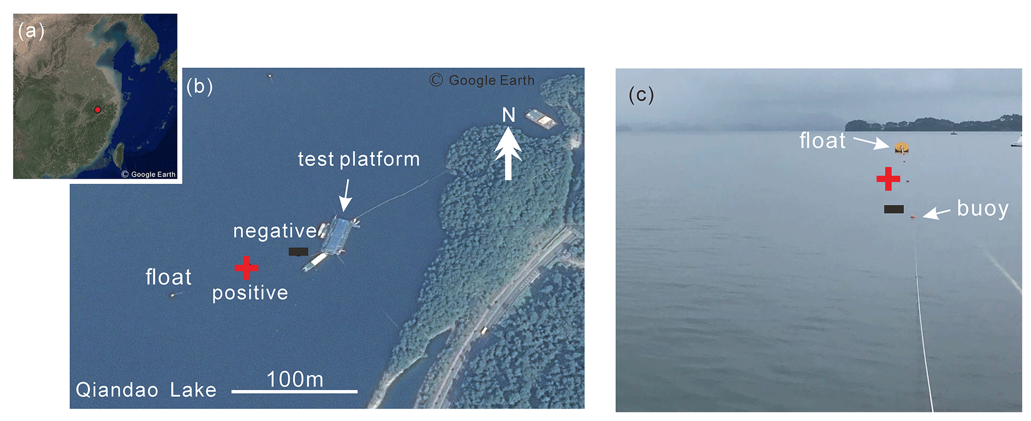
Figure 2Layout of the artificial SP source. (a) Location of Qiandao Lake (© Google Earth, 2019). (b) Position of the artificial source in the water (plan view) (© Google Earth, 2019). (c) Zoomed in location of the artificial source. Red plus and black minus signs denote the positive and negative poles of the DC power, respectively.
3.4 Data acquisition
Before the AUV entered the water, all electrodes were placed on the AUV system (as shown in Fig. 1). The AUV first dove to an 8 m depth at a constant speed and performed repeated measurements surrounding the positive and negative poles. The average speed of the AUV was about 1 kn (0.5 m s−1), and the sampling frequency of the electrical field sensors was 150 Hz. Other tests, including repeatedly switching the power on and off manually and changing the navigation speed and steering, were also conducted to determine the influence of the AUV body on the electrical field signal during navigation.
4.1 Noise analysis of the lake test
Sensors mounted on the AUV do not move with waves, but we detect obvious anomalies around active sources, and noises from the AUV are analyzed in this section. Figure 3 shows the three-component electrical field in water. The artificial source produced a stable electrical field similar to an electric dipole source in water. At the beginning of the test, the system was far away from the negative pole, and the collected electrical field was approximately equal to the background field. The amplitude fluctuated around 0 mV. When passing near the location of the artificial current source, the electrical field sensor could detect that the potential changed up to 30 mV. Because the system was always close to the negative electrode during the measurement process, the recorded electrical field was less affected by the positive pole or electrode.
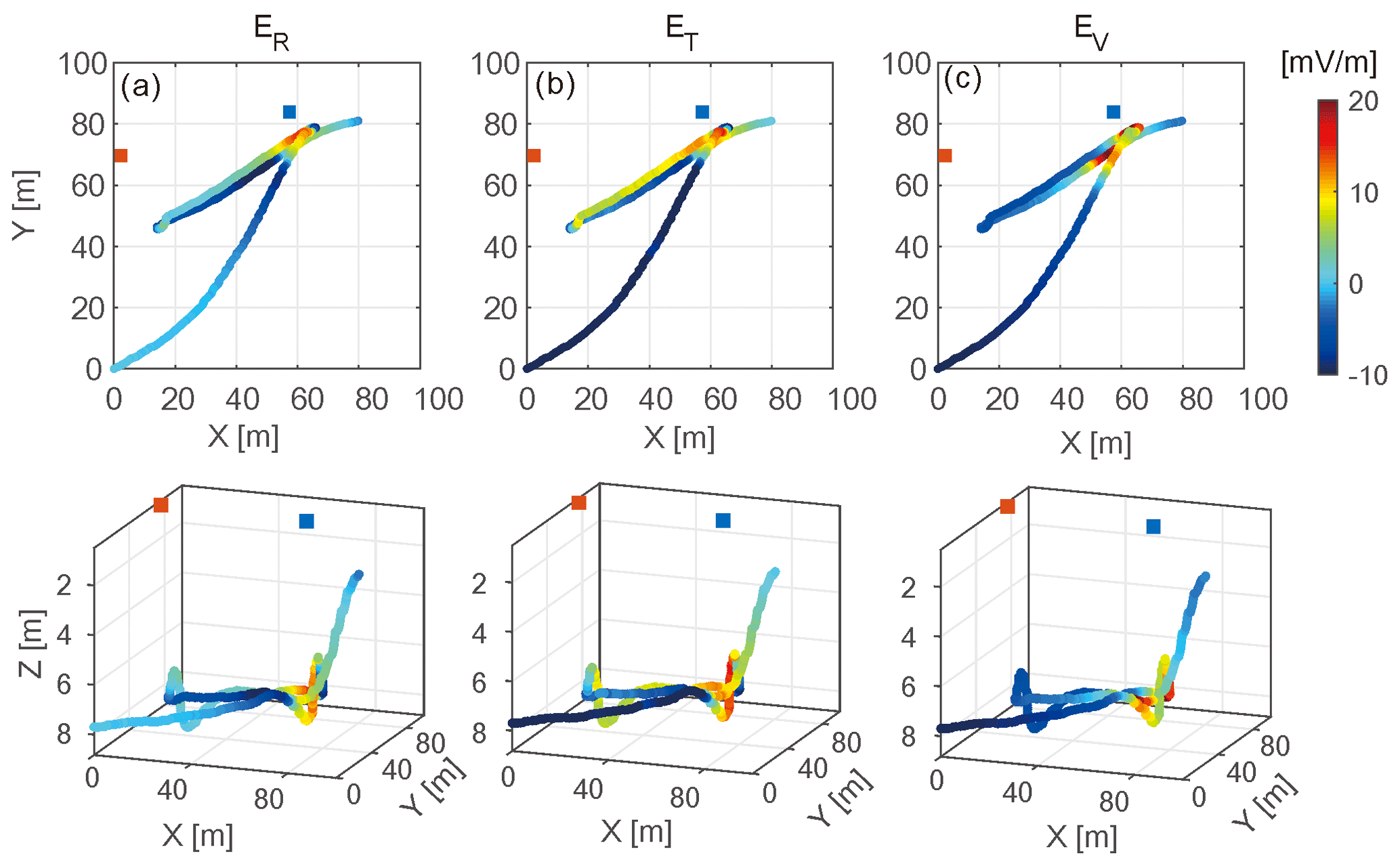
Figure 3The planar distribution of the three components of the electrical field measured by the AUV-based SP system (planar view in the upper panels, 3D view in the lower panels): (a) inline component of the electrical field, (b) crossline component of the electrical field, (c) vertical component of the electrical field. Red and blue dots represent the positive and negative poles of the artificial source, respectively.
In order to analyze the influence of the AUV body on the electrical field sensor, the frequency spectrum of the electrical field time series measured by the artificial current source was analyzed (we calculate the power spectrum of time series and convert the unit into dB by using log10(power)). Figure 4 shows the time series data of the three-component electrical field over a period of 15 min. The overall noise level was related to the position of the electrode. Results of power spectrum calculation showed the following characteristics:
-
the effective signal was mainly concentrated at low frequencies, and the noise level decreased with the increase in frequency,
-
the electrodes far from the AUV body had lower noise,
-
the noise of vertical component was lower than that of horizontal component,
-
except for the 50 Hz industrial interference, the peak values of the power spectrum were basically consistent with the rotation speed of propellers (1.4 Hz corresponds to a speed of 85 rpm, and peaks of 3.5–4.5 Hz correspond to a speed from 210 to 285 rpm).
In addition, the noise of 2.1 Hz corresponding to the vertical component was mainly caused by the vibration of the connecting rod in the water. The camera attached to the head of the connecting rod recorded the corresponding vibration image, providing a reference for improving the material and installation mode of the connecting rod.
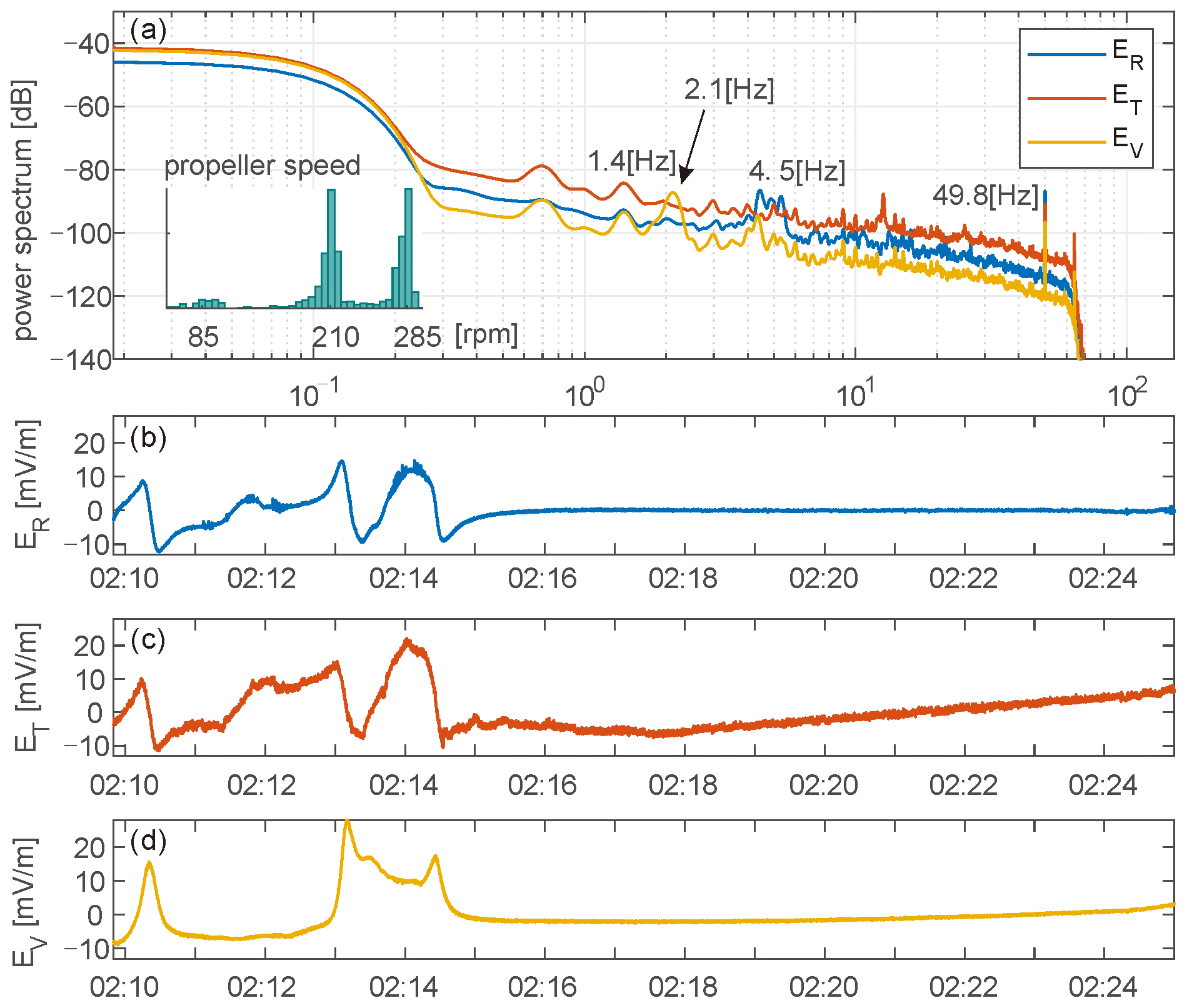
Figure 4Time series of the three components of the electrical field and the frequency analysis of the recorded data. (a) Spectrum of the three components of the electrical field with the histogram of propeller speed. The frequency components of 1.4 and 3.5–4.5 Hz are caused by the speed of propellers. The lower three panels show (b) the time series of the inline component ER, (c) the time series of the crossline component ET and (d) the time series of the vertical component EV.
4.2 AUV navigation attitude impact and correction
The attitude of the AUV has a significant impact on the SP data and therefore should be considered and corrected during field data processing and interpretation. The attitude angle in the local coordinate system is usually used to describe the attitude and spatial position of the AUV, including azimuth angle (heading), pitch angle and roll angle. The global reference coordinate system was determined according to the geodetic coordinates and the position of the survey lines. Following this, the relative relationship between the two coordinates was determined by the rotation of the coordinate system, as shown in Fig. 5c. The coordinate axis of the reference coordinate system is assumed to be (X0, Y0, Z0). The local coordinate system of the first rotation (X1, Y1, Z1) is obtained by rotating the azimuth angle H clockwise with Z0 as the rotation axis, then (X2, Y2, Z2) is obtained by rotating the pitch angle P clockwise with X1 as the rotation axis, and finally (X3, Y3, Z3) is obtained by rotating the roll angle R clockwise along the Y2 axis. The above procedure can be represented by three rotation matrices below. The electrical field that is supposed to be rotated in the reference coordinate system is Eg (Ex, Ey, Ez), and the measured electrical field in the local coordinate system after the rotation is Erot (ER, ET, EV), which gives us and in component form we have the following coordinates.
The corresponding inverse transformation is as follows:
The AUV avoids obstacles and steers according to changes in bathymetry when navigating over the seafloor. The electrical field Eobs recorded by the sensors attached to the AUV contains information about the navigation attitude. By ignoring acquisition noise and positioning errors, Eobs recorded by the AUV should be consistent with the rotated Erot. Whether the measured electrical field of the AUV is consistent with the electrical field generated by dipoles in uniform space is verifiable through numerical simulation.
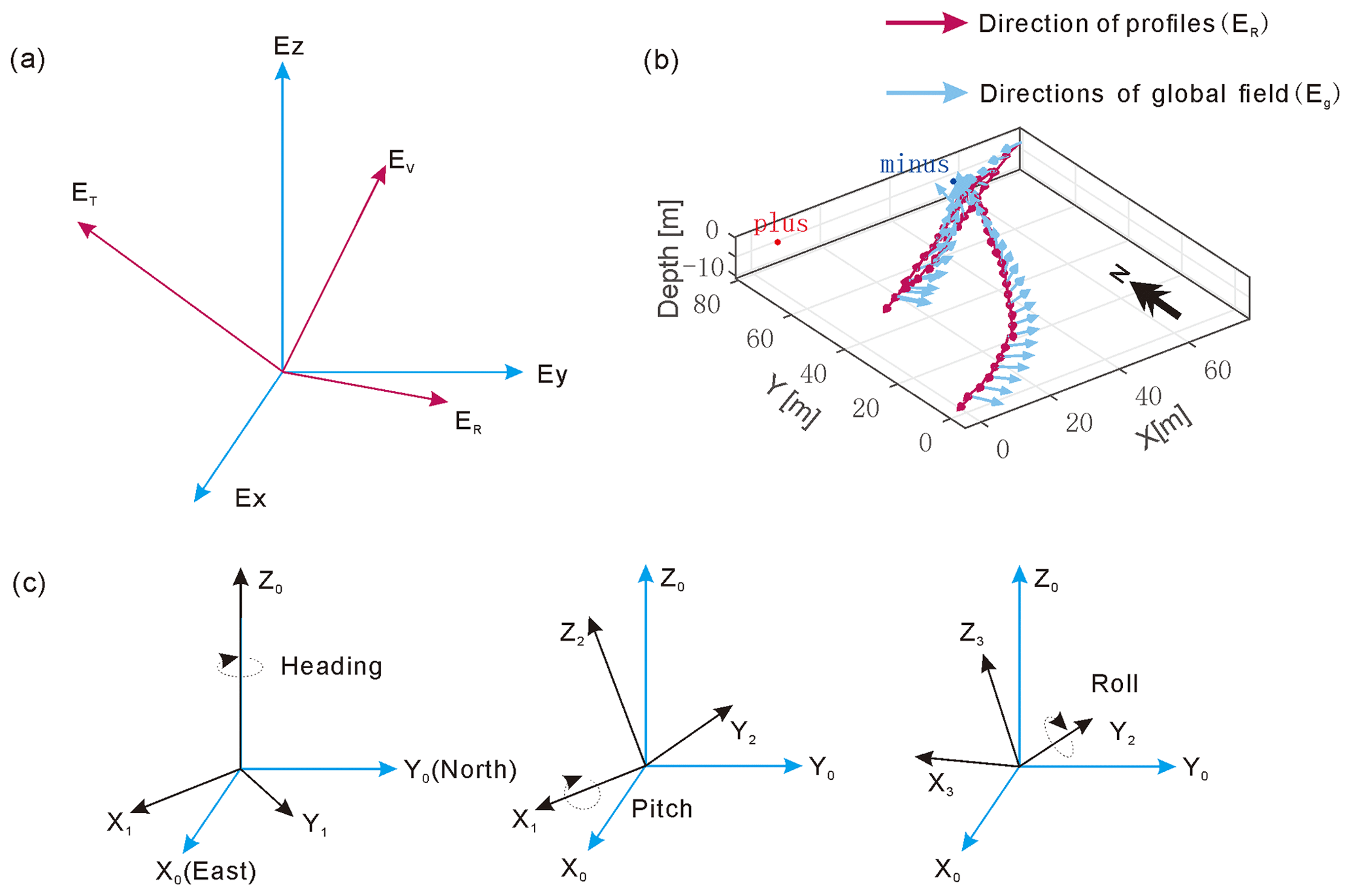
Figure 5Rotation relationship between the global electrical field Egand rotated electrical field Erot. (a) The projection of the global and rotated electrical fields in a Cartesian coordinate system. (b) The path of the AUV in the water; arrows denote the direction of AUV movement and the vector direction of the total electrical field in a geodetic coordinate system. Plus signs denote the position of positive pole, and minus signs denote the position of negative pole. (c) Definition of the different attitude angles.
Based on the situation of the lake test, a three-dimensional (3D) model of 100 m × 100 m × 30 m was established in the Cartesian coordinate system, where positive and negative poles of the dipole were located at (3, 75, −1) and (54, 80, −0.5), respectively. The 3D model was discretized into unstructured grids, the Poisson equation of the steady-state current field was solved by the finite-element method, and boundary conditions of the first kind were used at the bottom of the lake. The global electrical field Eg (Ex, Ey, Ez) was extracted according to AUV location data, and then the electrical field in the local coordinate system along the direction of profile was denoted as Erot(ER, ET, EV) and calculated using Eq. (1). Field data measured by the AUV were denoted as Eobs (ER, ET, EV). The relationship between global Eg (Ex, Ey, Ez) and local Erot (ER, ET, EV) is shown in Fig. 5b. When the AUV is moving from south to north, the observation field is in the same direction as the reference field and vice versa when the AUV is moving from north to south.
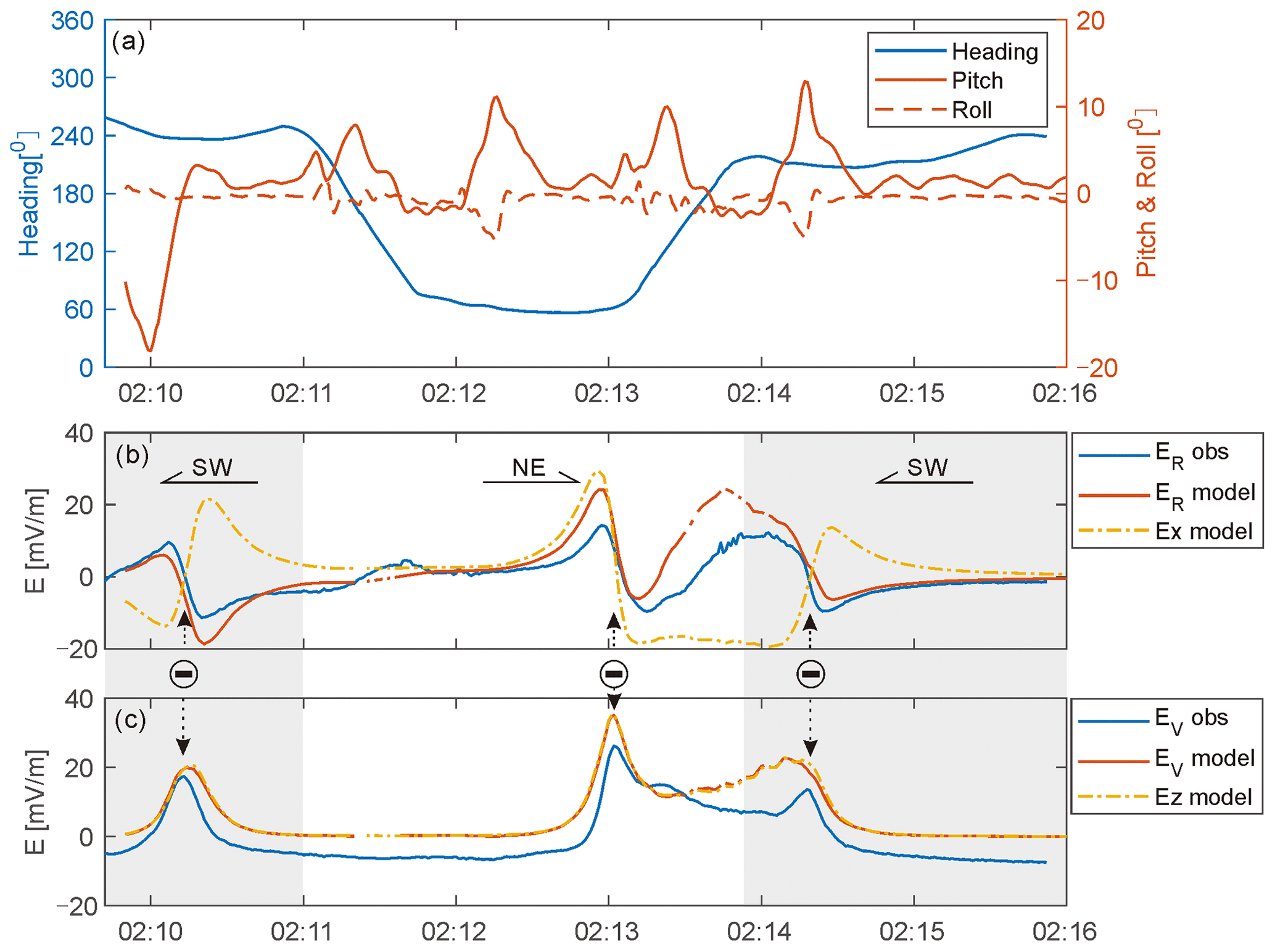
Figure 6Comparison of the measured data and numerical simulation: (a) navigation attitude of the AUV in the water; (b) time series of modeled and observed horizontal components with different travel directions; and (c) modeling and observed vertical component for SW, NE, and SW profiles. Minus signs correspond to the location of negative pole of the artificial source.
The attitude of the AUV is shown in Fig. 6a. The AUV navigated stably in the lake, and the roll angle was less than 5∘. The pitch changed when the vehicle was rising or falling, and the overall pitching angle was less than 20∘. In the measured range shown in Fig. 6a, the vehicle changed direction twice at 02:11 and 02:14 GMT, respectively. The measured and simulation results in Fig. 6b and c showed that the attitude of the AUV has different impacts on each component of the electrical field. Specifically, the azimuth has significant influence on the horizontal component of the electrical field but has little influence on the vertical component. When the survey line went along the SW direction, the variation trend of ER along the survey line (solid red line in Fig. 6b) and global component Ex were opposite; when the survey line went along the NE direction, ER and Ex changed in the same direction. After rotation correction, the observation data of the submersible were basically consistent with the simulation results. The position where the gradient of the horizontal electrical field component changed the most significantly corresponded to the negative pole of the artificial source. Azimuth has little effect on the vertical component because the AUV was always below the negative source and the electrical field direction pointed up. Therefore, the change in azimuth angle will not change the direction of the vertical component. In addition, because the pitch angle was very small and the attached electrode was basically maintained in the vertical state, the vertical component of the measured electrical field EV was approximately equal to that of the global component EZ.
The forward problem of SP can be expressed by a Poisson equation of potential (Jardani et al., 2008):
where ℑ is the volumetric current density (A m−3), Js is the current density vector (A m−2), σ is the conductivity (S m−1), E is the electrical field vector and V represents the SP field.
By changing the source term of Eq. (3), the SP response to various effects can be calculated, such as the flow potential related to groundwater flow (Ahmed et al., 2013) or the geobattery model related to polymetallic deposits (Rittgers et al., 2013).
In order to investigate the reliability and interpretability of electrical field data measured by the AUV-SP system, the regularized least-squares method was applied for the inversion of the artificial SP source. Assuming that m is the bulk current density model vector and m0 is the reference model, the inversion can be expressed as the minimization of the following objective function:
where Wd is the data-weighting matrix and Δd is the difference between the data d obtained by forward modeling and the observed data dobs, also known as data residual. Here, the measured electrical field component is selected as the observation data, W is the model-weighted diagonal matrix, and α is the regularization factor. The regularization factor α was used to balance the model constraints and data-fitting function in the process of solving the model. It can be determined by the L-curve criterion (or generalized cross-validation method) or by experience. Because the electrical field decays rapidly with distance, the inversion of the seafloor SP data only gives a shallow current density distribution, which cannot accurately reflect the situation of the space current dipole source under the seafloor. Therefore, it is necessary to introduce a depth-weighting function to enhance the sensitivity of the grid element far from the observation point. The depth-weighting function Wz should be placed in the model constraints as follows (Biswas and Sharma, 2017; Portniaguine and Zhdanov, 1999):
where Wj is the jth element on the main diagonal of matrix Wz and J is the sensitivity matrix (or Jacobian matrix). M is the number of model vector elements, and N is the number of the observation point. The p value is constant and generally equal to 1. The extent of depth weighting can be adjusted by the value of p. For multicomponent inversion, the full three-component electrical field were used and the total amount of observation data became 3×N.
In application, the SP data can be inverted in many ways to determine the flow direction of the fluid or the location of the self-potential source. When the source location is to be solved, it was usually assumed that the conductivity distribution in the space is known or determined by other electrical exploration methods (DC conductivity or induction-based electromagnetic methods), and thus the SP source is equivalent to the external current source. Therefore, this study used the inverted volumetric current density distribution to locate the simulated artificial source. On land, the SP method usually directly measures the electric potential between the roll electrode and a fixed electrode; therefore, the potential data V are directly chosen for inversion. However, in the marine environment, it is impossible to fix a reference electrode on the seafloor when the ship or AUV is moving. Therefore, the SP method conducted in the marine environment usually measures the gradient of electric potential, i.e., the electrical field, and the potential is calculated indirectly by numerical integration. In the case of this study, the measured electrical field components were directly inverted.
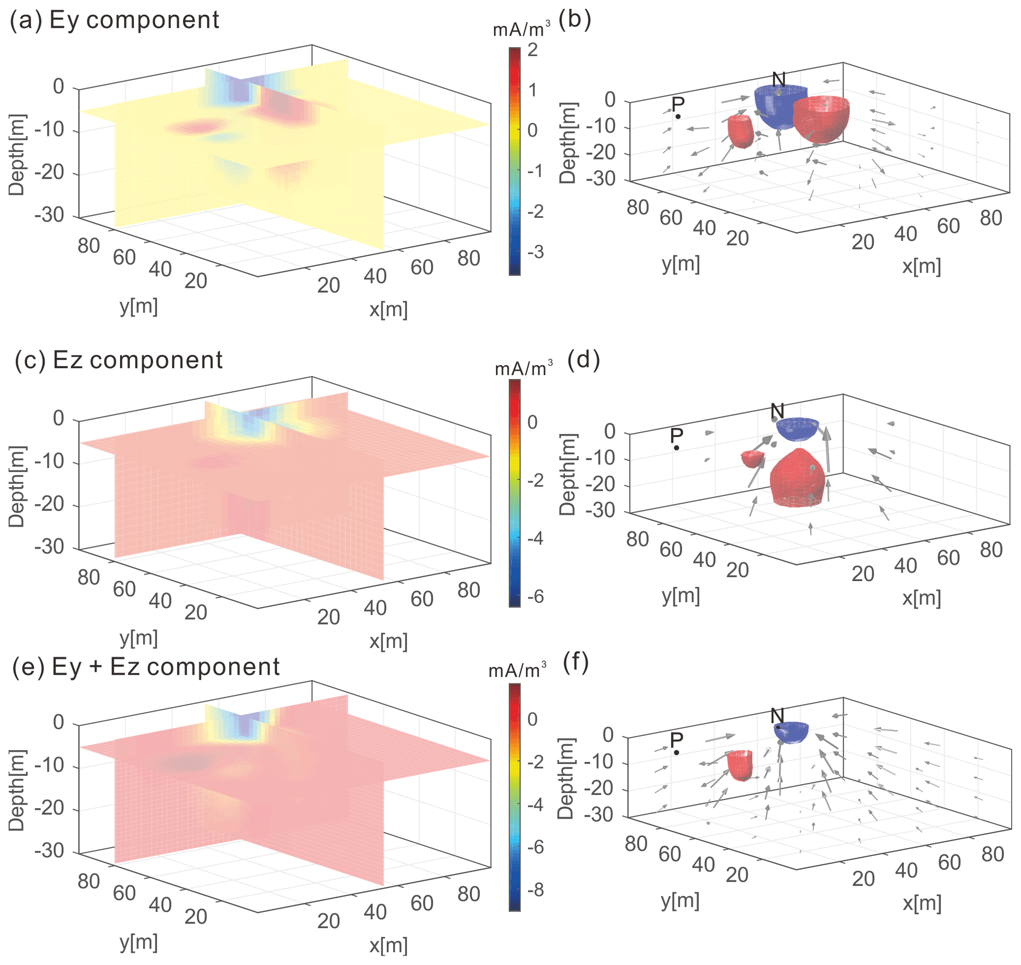
Figure 7Volumetric current density inversion results of different components of observed data, with p=1 and α=0.01. Panels (a) and (b) show the inversion results of volumetric current density of horizontal components of electrical field data (magnitude and direction). Panels (c) and (d) show the inversion results of the charge density of the vertical component of observed data (magnitude and direction). Panels (e) and (f) the inversion results of the charge density of both components of the observed data (magnitude and direction). The arrow direction indicates the diffusion direction of the current density. The intersection of the vertical section is the position of the negative pole of the artificial source. Although the anomaly recovery for a single component can also localize the negative pole, the two-component inversion returns a single compact current density. The notation P corresponds to the location of the positive pole of the artificial source. The notation N corresponds to the location of the negative pole.
Owing to the limited observation data collected by the AUV-SP system near the artificial source, the inversion result is nonunique. Therefore, the constraints of known information, such as the lake water conductivity (1 S m−1, measured with the environment sensor from the AUV) and lake bottom sediment conductivity (assumed to be 0.1 S m−1), were added to the inversion. To investigate the advantages of multicomponent inversion, single-component and two-component observation data were used for the inversion and the inversion results were compared. Figure 7 shows the results obtained by inversion of electrical field data of a single component (horizontal component and vertical component, Fig. 7a and b, respectively) and two components (horizontal component and vertical component, Fig. 7c) under the same constraint conditions. Negative charge density was recovered surrounding the negative pole of the artificial source in all results, which preliminarily revealed the reliability of the system and the effectiveness of the inversion method. Indeed, because the AUV-SP system's navigation path in the lake is mainly near the negative pole of the artificial source, the negative pole position of the artificial source can be precisely located, while positive pole is not easily located due to the lack of observation data of the surrounding area, although some positive charge density is retrieved along the survey line. By comparing the inversion results between a single component (Fig. 7a and b) and multiple components (Fig. 7c), it was observed that the inversion results of the two horizontal components of the electrical field were more focused, and the negative charge intensity was concentrated, while the negative charge density obtained from the inversion results of the single vertical component of the electrical field was accompanied by positive charge anomaly, which dispersed the negative charge energy and deviated from the actual situation. Combinations of vertical and horizontal components of electrical field data restrict the horizontal distribution of charge density and make the inversion more consistent with the actual artificial source. In addition, the current flow direction (Fig. 7b, d, f) also shows that the inversion of only a single component will produce the wrong current direction and that additional constraints (e.g., boundary limits, heterogeneous distribution of conductivity) were required to obtain reasonable inversion results. Therefore, multicomponent detection of electrical field is necessary when addressing complex geological structure, especially involving flow of fluids.
A seafloor SP measurement system that consisted of three pairs of perpendicular electrodes attached to the AUV (Qianlong 2) was introduced. By deploying an artificial current source, the multicomponent electrical field responses in the water were measured by the AUV in Qiandao Lake. The observed results were consistent with the numerical simulation, which verifies the feasibility of the AUV-SP system for multicomponent SP exploration. At present, the AUV-SP system can work in water for about 40 h and complete the SP measurement of a high-resolution area of about 20 km2.
The test results of two surveys showed that the AUV-SP system has good consistency and repeatability and that the overall noise level of the measured data is relatively low, which meets the requirements of near-seafloor SP exploration at a large scale. The inversion of the test data of the AUV-SP system demonstrated that the position and intensity of the inverted current source were basically consistent with the actual position and intensity of the artificial current source. Therefore, the SP response measured by the AUV-SP system can be used to locate the seafloor SP source to achieve an accurate exploration and evaluation of seafloor sulfide deposits. In the case of simple geoelectric structure, a single vertical component measurement would be sufficient to locate the SP source, but in solving complex problems such as hydrothermal or fluid flow, a three-component SP measurement is crucial.
In view of the vibration noise of the connecting rod presented in this test, our next step will be to select a more suitable material and design a bracket with better rigidity to reduce the vibration noise. The experience and data accumulated in this experiment also provide a reference for the future research of active-source electromagnetic detectors on AUVs.
The code for the processing is available upon request (591149254@qq.com).
The raw data from the experiments are available upon request (591149254@qq.com).
ZZ processed the data and wrote the paper. JS was the project leader. CT provided ideas and designed the AUV-SP system,. XD, TW, ZN and WW tested the system together. ZS proofread the manuscript.
The authors declare that they have no conflict of interest.
The authors thank the China University of Geosciences (Beijing) for providing the data acquisition device and electrodes.
This work was supported by National Key R&D Program of China (contract nos. 2018YFC0309901, 2017YFC0306803) and China Ocean Mineral Resources R&D Association (COMRA; contract nos. DY135-S1-1-01, DY135-S1-1-07).
This paper was edited by Lev Eppelbaum and reviewed by Kai Chen and two anonymous referees.
Ahmed, A. S., Jardani, A., Revil, A., and Dupont, J. P.: SP2DINV: A 2D forward and inverse code for streaming potential problems. Comput. Geosci., 59, 9–16, https://doi.org/10.1016/j.cageo.2013.05.008, 2013.
Biswas, A. and Sharma, S. P.: Interpretation of self-potential anomaly over 2-D inclined thick sheet structures and analysis of uncertainty using very fast simulated annealing global optimization, Acta Geod. Geophys., 52, 439–455, https://doi.org/10.1007/s40328-016-0176-2, 2017.
Cherkashev, G. A., Ivanov, V. N., Bel Tenev, V. I., Lazareva, L. I.,Rozhdestvenskaya, I. I., Samovarov, M. L., Poroshina, I. M., Sergeev, M. B., Stepanova, T. V., and Dobretsova, I. G.,: Massive sulfide ores of the northern equatorial Mid-Atlantic Ridge, Oceanol., 53, 607–619, https://doi.org/10.1134/S0001437013050032, 2013.
Constable, S., Kowalczyk, P., and Bloomer, S., Measuring marine self-potential using an autonomous underwater vehicle, Geophys. J. Int., 215, 49–60, https://doi.org/10.1093/gji/ggy263, 2018.
Corry, C. E.: Spontaneous polarization associated with porphyry sulfide mineralization, Geophysics, 50, 1020–1034, https://doi.org/10.1190/1.1441967, 1985.
Corwin, R. F.: Offshore Application of Self-potential Prospecting, Scripps Institution of Oceanography Library, 1973.
Corwin, R. F.: Offshore use of the self-potential method, Geophys. Prospect., 24, 79–90, https://doi.org/10.1111/j.1365-2478.1976.tb00386.x, 1976.
Eppelbaum, L. V.: Advanced analysis of self-potential field analysis in ore deposits of the South Caucasus, Proceedings of the National Azerbaijan Academy of Sciences, 2, 21–35, https://doi.org/10.33677/ggianas20190200029, 2019.
Eppelbaum, L. V.: Quantitative analysis of self-potential anomalies in archaeological sites of Israel: an overview, Environ. Earth Sci., 79, 1–15, https://doi.org/10.1007/s12665-020-09117-w, 2020.
Fox, R. W.: On the electromagnetic properties of metalliferous veins in the mines of Cornwall, Philos. T. R. Soc. Lond., 120, 399–414, 1830.
Heinson, G.: Marine self potential exploration, Expl. Geophys., 30, 1–4, https://doi.org/10.1071/EG999001, 1999.
Jardani, A., Revil, A., Bolève, A., and Dupont, J. P.: Three-dimensional inversion of self-potential data used to constrain the pattern of groundwater flow in geothermal fields, J. Geophys. Res., 113, B09204, https://doi.org/10.1029/2007JB005302, 2008.
Kawada, Y., Kasaya, T.: Marine self-potential survey for exploring seafloor hydrothermal ore deposits, Sci. Rep.-UK 7, 1–12, https://doi.org/10.1038/s41598-017-13920-0, 2017
Kawada, Y., and Kasaya, T.: Self-potential mapping using an autonomous underwater vehicle for the Sunrise deposit, Izu-Ogasawara arc, southern Japan, Earth, Planets and Space, 70, 142, https://doi.org/10.1186/s40623-018-0913-6, 2018.
Komori, S., Masaki, Y., Tanikawa, W., Torimoto, J., Ohta, Y., Makio, M., Maeda, L., Ishibashi, J., Nozaki, T., Tadai, O., and Kumagai, H.: Depth profiles of resistivity and spectral IP for active modern submarine hydrothermal deposits: a case study from the Iheya North Knoll and the Iheya Minor Ridge in Okinawa Trough, Japan, Earth Planet Space, 69, 114 https://doi.org/10.1186/s40623-017-0691-6, 2017.
Naudet, V. and Revil, A.: A sandbox experiment to investigate bacteria-mediated redox processes on self-potential signals, Geophys. Res. Lett., 32, L11405, https://doi.org/10.1029/2005GL022735, 2005.
Portniaguine, O. and Zhdanov, M. S.: Focusing geophysical inversion images, Geophysics, 64, 874–887, https://doi.org/10.1190/1.1444596, 1999.
Revil, A., Finizola, A., Piscitelli, S., Rizzo, E., Ricci, T., Crespy, A., Angeletti, B., Balasco, M., Barde Cabusson, S., Bennati, L., Bolève, A., Byrdina, S., Carzaniga, N., Di Gangi, F., Morin, J., Perrone, A., Rossi, M., Roulleau, E.,and Suski, B,: Inner structure of La Fossa di Vulcano (Vulcano Island, southern Tyrrhenian Sea, Italy) revealed by high-resolution electric resistivity tomography coupled with self-potential, temperature, and CO2 diffuse degassing measurements, J. Geophys. Res.-Sol. Ea., 113, B07207, https://doi.org/10.1029/2007JB005394, 2008.
Rittgers, J. B., Revil, A., Karaoulis, M., Mooney, M. A., Slater, L. D., and Atekwana, E. A.: Self-potential signals generated by the corrosion of buried metallic objects with application to contaminant plumes, Geophysics, 78, EN65-EN82, https://doi.org/10.1190/geo2013-0033.1, 2013.
Safipour, R., Hölz, S., Halbach, J., Jegen, M., Petersen, S., and Swidinsky, A.: A self-potential investigation of submarine massive sulfides, Palinuro Seamount, Tyrrhenian Sea, Geophysics, 82, A51–A56, https://doi.org/10.1190/geo2017-0237.1, 2017.
Sato, M. and Mooney, H. M.: The electrochemical mechanism of sulfide self-potentials, Geophysics, 25, 226–249, https://doi.org/10.1190/1.1438689, 1960.
Sudarikov, S. M. and Roumiantsev, A. B.: Structure of hydrothermal plumes at the Logatchev vent field, 14 45′ N, Mid-Atlantic Ridge: evidence from geochemical and geophysical data, J. Volcanol. Geoth. Res., 101, 245–252, https://doi.org/10.1016/S0377-0273(00)00174-8, 2000.
Tao, C., Xiong, W., Xi, Z., Deng, X., and Xu, Y.: TEM investigations of South Atlantic Ridge 13.2 S hydrothermal area, Acta Oceanol. Sin., 32, 68–74, https://doi.org/10.1007/s13131-013-0392-3, 2013.
Wu, T., Tao, C., Zhang, J., Wang, A., Zhang, G., Zhou, J., and Deng, X.: A hydrothermal investigation system for the Qianlong-II autonomous underwater vehicle, Acta Oceanol. Sin., 38, 159–165, https://doi.org/10.1007/s13131-019-1408-4, 2019.
- Abstract
- Introduction
- AUV-based SP system
- Lake test design and data acquisition of the AUV-based SP system
- Results and analysis
- Inversion scheme of the AUV-based self-potential data
- Conclusions
- Code availability
- Data availability
- Author contributions
- Competing interests
- Acknowledgements
- Financial support
- Review statement
- References