Experimental analysis of Taylor bubble regimes using kymography: a tool for understanding bubble ascent dynamics in open-vent volcanic conduits

Taylor bubbles, or gas slugs, are elongated gas pockets that drive discrete and cyclic Strombolian explosions. To understand the surface dynamics of such eruptions, it is essential to first characterize the subsurface flow behaviour within the shallow (< 1 km) volcanic plumbing system. This can be achieved experimentally by simulating Taylor bubble flow under conditions that are mathematically scalable to volcanic conduit settings. This paper presents a novel application of kymography – an existing visual analysis technique – for measuring isolated or continuous Taylor bubble flow experimentally in vertical cylindrical pipes. Kymographs condense thousands of frames of experimental footage into a single space-time image, enabling efficient analysis of flow dynamics. The method utilises open-source software (ImageJ), affordable experimental equipment, and straightforward calibration, making it both cost-effective and widely accessible. Here, we illustrate the value of incorporating kymography to simplify and enhance data retrieval from complex two-phase fluid problems which provide a rigorous first-order understanding of the flow processes governing surface eruption dynamics exhibited by open-vent basaltic volcanoes. We show that kymography serves as a valuable and effective visual analysis tool for the experimental measurement of gas volume fraction, gas and liquid slug velocities, bubble length and diameter, falling film thickness, bubble and coalescence event counts, and to indicate steady-state ascent. In a volcanic conduit, these parameters have important implications for flow stability, interaction dynamics, overpressure development, and the volume of gas released at burst, which ultimately aids our ability to understand and predict eruption style, periodicity, repose, and explosivity level.

1 Background

1.1 Bubble-driven volcanic eruptions & other Taylor bubble phenomena

Low viscosity volcanic systems exhibit a variety of eruption styles with variable intensities within short time periods (Gaudin et al., 2017). Eruption dynamics are primarily driven by the ascent and burst dynamics of gas from within volcanic conduits. Characterising the fluid dynamics of gas bubbles as they ascend within the conduit – particularly their morphologies, velocities, and interaction behaviours – is critical in improving our understanding of surface explosivity and eruptive style transitions. Since we cannot directly observe the inner workings of a volcano, the mechanisms of bubble formation, interaction, and ascent are inferred using observations of eruptions visible at the surface, samples of erupted material, and laboratory experiments designed to imitate known volcanic conditions. Much of what is known about the flow dynamics inside volcanic conduits comes from an extensive series of experimental studies designed to closely replicate in-conduit behaviours in conditions that are safe, controlled, and quantifiable. In the simplest terms, we can think of a basaltic open-vent volcanic conduit as a kilometres-long cylindrical transport pathway for magma and a separated phase of buoyantly ascending bubbles, where eruptions occur as a result of these bubbles bursting at the free magma surface. Indeed, many models for volcano-scale in-conduit fluid dynamics attribute specific eruptive activity to a series of regimes that are also recognisable in two-phase pipe flow in the engineering literature (Vergniolle and Jaupart, 1986). These distinctive bubble morphologies are attributed to specific expressions of surface activity, as shown in Fig. 1, of which there are three broad classifications: passive, effusive, and explosive activity. Passive degassing typically involves low gas volume fractions (GVFs) of small spherical or ellipsoid/deformed bubbles emerging from open-vent conduits, lava lakes, or fumaroles. Effusive activity involves the outflow of lava sometimes accompanied by low-level explosive activity, coming from individual or multiple vents. The transition from effusive to explosive activity can occur gradually or rapidly (James et al., 2008; Maruishi and Toramaru, 2024; Parfitt and Wilson, 1995), and increasing bubble size significantly increases the possibility that more explosive activity is produced (James et al., 2009).

Figure 1 Example flow regimes and the surface eruption styles to which they are attributed. These regimes can be present in tubes at the laboratory scale and in volcanic conduits. Image is adapted from Lehr and Rabbel (2021) and Pering et al. (2017).

A key factor in the shift from passive or effusive to explosive behaviour is the formation of Taylor bubbles (also known as slugs). Taylor bubble formation begins with the exsolution of a limited gas volume from the melt as pressure decreases towards the surface (Gardner et al., 2022; Sparks, 1978). The exsolved bubbles remain small and compressed until the amount of gas and the surrounding pressure reaches a critical value and bubbles decouple from the magma and rise as a separate phase (James et al., 2004). Small spherical or slightly elongated or deformed bubbles transition into spherical cap and Taylor bubble morphologies by expansion-driven coalescence (Parfitt, 2004; Parfitt and Wilson, 1995), or as a result of the sudden collapse of an accumulated foam layer (Jaupart and Vergniolle, 1989). The bubble diameters become close to conduit (diameter)-filling, with morphologies that can be characterised by the presence of a nose, body and base, or tail, with a surrounding liquid falling film and trailing liquid wake (Llewellin et al., 2012). This change in bubble morphology drives a transition in flow regime to the extent that their governing fluid dynamics also change, and the conduit diameter (in addition to the pre-existing characteristics of the host magma) becomes a major control on bubble ascent. Taylor bubbles are classified as such when their length is greater than 1.5 times the surrounding conduit diameter (Llewellin et al., 2012; Shosho and Ryan, 2001), or when the surrounding liquid falling film has a length larger than or equal to the surrounding conduit diameter (Davies and Taylor, 1950). The ascent of single Taylor bubbles occurs due to sporadic releases of limited gas volumes into the conduit, and continuous Taylor bubble flow occurs due to moderate rates of continuous gas release (Seyfried and Freundt, 2000).

Taylor bubbles are most known in volcanology as the drivers of discrete and cyclic VEI 1–3 (mild to moderate) Strombolian explosions that are archetypal to Stromboli, but also observed at Etna, Yasur, Pacaya, and Erebus, among others. Strombolian explosions are one of the most widespread expressions of uninterrupted basaltic sub-aerial volcanism globally (Pering et al., 2016; Pering and McGonigle, 2018). Experimental studies of two-phase flow in conditions that are scalable to volcanic systems are the key to understanding the in-conduit flow dynamics driving these explosions because they facilitate the measurement of key bubble and liquid flow parameters (e.g., bubble velocity, bubble morphology, falling film thickness, and coalescence processes). These parameters influence the overall stability of the flow, the interaction dynamics between bubbles, the circulation dynamics of magma within the conduit, and the volume of gas released at burst, which ultimately enhances our understanding of the mechanisms for eruption periodicity, repose, explosivity, and the transitions between eruptive styles. Indeed, our current knowledge of the fluid dynamics of Taylor bubbles within volcanic conduits – whether ascending in isolation or within a train – is built upon an extensive foundation of experimental studies (Table 1). Taylor bubbles are a subject of broad interdisciplinary interest in both research and industry (Morgado et al., 2016). Outside of volcanology, Taylor bubble flow is relevant to the study of microfluidics and capillary flows (Etminan et al., 2021), buoyancy-driven fermenters, production and transportation of hydrocarbons in the oil and gas industry (Ambrose, 2015), emergency cooling of nuclear reactors, and the boiling and condensing processes in thermal power plants (Aql and Al-Safran, 2024). Understanding how Taylor bubbles flow in pipes is important to many fields, and thus their accurate measurement and analysis is essential. By refining our ability to measure and interpret the experimental dynamics of Taylor bubbles under conditions that suitably scale volcanically, we can improve our capacity to anticipate transitions in eruption behaviour.

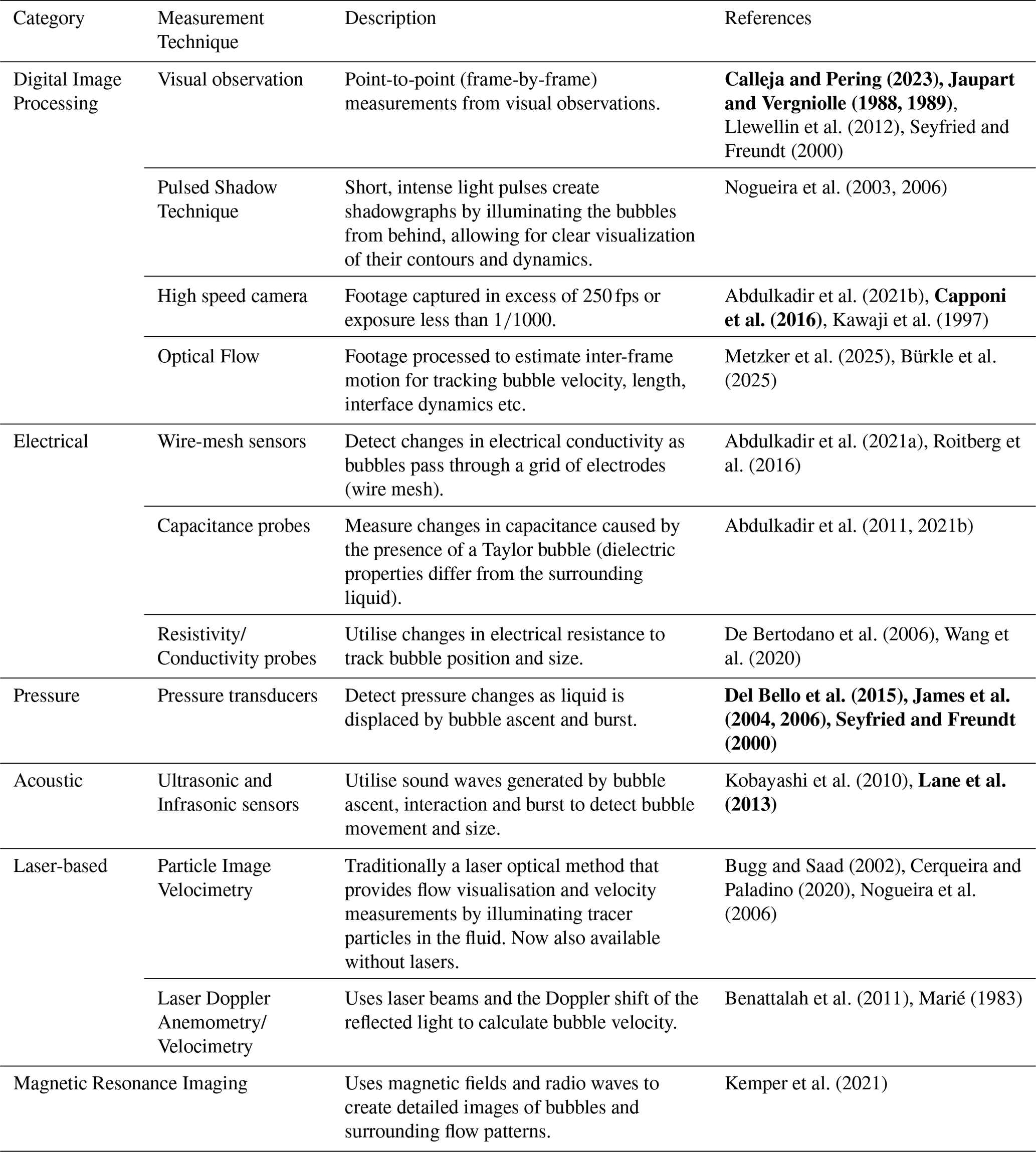
Table 1 Existing techniques for the measurement of experimentally generated Taylor bubble flow with example references for each. Bold references indicate studies that investigate volcanic Taylor bubble flow.

1.2 Experimental measurement of Taylor bubbles

In volcanology, the key parameters of interest surrounding Taylor bubble ascent are investigated for their role in governing flow-conditions and ultimately surface eruption dynamics. These parameters include gas volume fraction, gas and liquid slug velocities, bubble length and diameter, falling film thickness, bubble frequency, and the tracking of coalescence or break-up events. The most commonly used experimental techniques for the measurement of Taylor bubble parameters both within and outside of volcanology are described in Table 1. A review of these is also available in Calleja and Pering (2023).

Non-intrusive optical methods such as high-speed imaging, visual observations, and the pulsed shadow technique are typically used to track bubble ascent velocity and morphology in transparent media (Calleja and Pering, 2023; Jaupart and Vergniolle, 1988, 1989; Llewellin et al., 2012; Seyfried and Freundt, 2000). Traditional laser-based approaches like particle image velocimetry (PIV, now widely available as a digital image processing method without lasers) and laser doppler anemometry (LDA) enable precise velocity field and bubble interface measurements using tracer particles. These techniques are more accessible and offer non-intrusive methods for acquiring data at high spatial resolutions. However, their use is limited to transparent media (Calleja and Pering, 2023), and analysis can be computationally intensive at high frame rates. Electrical methods such as wire-mesh sensors and capacitance probes are commonly used to quantify bubble frequency, velocity, and length in opaque systems. These techniques provide real-time data at a low cost, and function well under a wide range of pressure and temperature conditions. However, their reliance on fluid conductivity to function means they are highly sensitive to environmental change and thus require regular recalibration; they are also ineffective in non-conductive fluids and need to be in direct contact with the flow to function. Pressure transducers provide time-resolved measurements of the pressure fluctuations associated with bubble ascent and bursting, while acoustic methods capture bubble dynamics through sound emission; these techniques are useful in optically inaccessible setups. Both methods are sensitive to noise or interference, and have reduced accuracy for bubble size measurements, but are capable of generating high accuracy velocity measurements. They have a wide application range including in extreme environments, and are used in the volcanic literature to experimentally link Taylor bubble ascent velocity and burst dynamics with pulsatory Strombolian eruption dynamics (Del Bello et al., 2015; Seyfried and Freundt, 2000). Magnetic resonance imaging (MRI) provides a 3D reconstruction of internal flow structure but is limited in application by its high cost and low temporal resolution.

We present a novel application of kymography – an existing digital image analysis technique – as an approach that is well-suited to measuring experimental Taylor bubble flow parameters such as gas volume fraction, gas and liquid slug velocities, bubble length and diameter, falling film thickness, bubble frequency, and to track coalescence or break-up events.

1.3 Kymographs

Kymographs – also referred to as time-space plots, dynamic motion analysis plots, rise diagrams, motion-track diagrams, or simply as a reslice – are a way to represent dynamic processes as time-space data in a single image. They are often applied to the visualisation of micron-scale dynamic processes in disciplines outside of volcanology wherein parameters such as the direction, speed, fluxes, and growth dynamics of the object/s of interest can be characterised. Examples include tracking the formation, division, growth, and geometry of cellular components (Mangeol et al., 2016), characterising velocity fields in microflows (Le and Fenech, 2022) and flow characterisation in porous media (Browne et al., 2020; Haward et al., 2021; Pak et al., 2018). In the Earth sciences, traditional kymographs (specifically a revolving paper-wrapped drum on which a stylus recorded motion changes over time) were used in seismography. In contemporary volcanology, kymographs are used to parameterise the frequency, height, and duration of both explosive and effusive eruptions, and to illustrate surface activity transitions over time e.g., for volcanic jets (Eibl et al., 2023; Muñoz et al., 2022; Spina et al., 2023; Taddeucci et al., 2023; Walter et al., 2023), gas emissions (Gaudin, 2017; Vossen et al., 2024), or ash plumes (Walter et al., 2020). Kymographs are also used to capture flow propagation and characterise coherent structures in pyroclastic density currents (Penlou et al., 2023; Trolese et al., 2024; Uhle et al., 2024).

In this paper we demonstrate, for the first time, the use of kymography as an effective digital image processing tool for the analysis of experimental Taylor flow in the context of Taylor bubble-driven volcanism. While kymography does not directly measure physical parameters e.g., pressure or acoustic variations, it effectively captures the motion of Taylor bubbles via identifiable flow features that facilitate the measurement of key flow parameters. Against the backdrop of existing techniques (Table 1), kymography offers a low-cost, accurate, and accessible visualisation tool that is complementary to sensor-based methods but can also be utilised as a stand-alone method in its own right.

2 Methods

2.1 Experimental setup

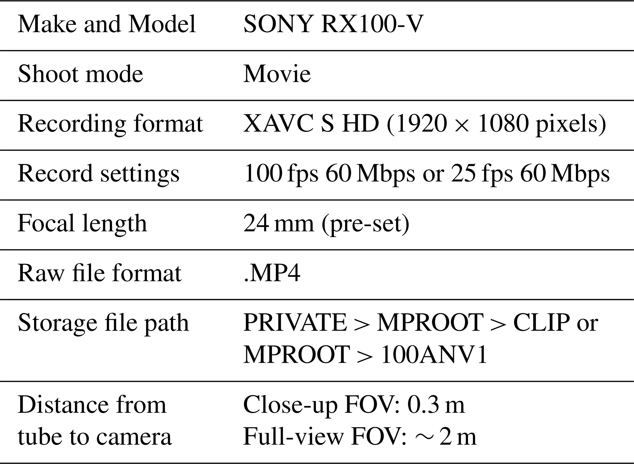
The basic setup (Fig. 2) is a simple and cost-effective gas injection system (Calleja and Pering, 2023) consisting of a transparent, vertical, open-ended tube (internal diameter (D): 0.036 m) filled with Newtonian fluids (water-glycerol mixtures, viscosity range: 0.001–0.79 Pa s). The tube is fitted with a voltage-controlled air pump that is capable of varied injection volumes (∼ 0.05–0.25 GVF), all of which form Taylor bubble flow regimes under the listed conditions (Table 2). Gas ascent is recorded against a white background with a SONY RX100-V compact camera at 25 and 100 frames per second (fps), where the camera field of view (FOV) captures a full view of the entire 1.75 m tube length, or a higher resolution close-up view of a 0.15 m segment, respectively. See Table A1 for specific camera settings. With the exception of water, our experimental conditions can be mathematically scaled to represent the low-viscosity basaltic systems that are commonly associated with Strombolian-style volcanism using dimensionless parameters (Table 2). The principle of dimensionless scaling lies in the assumption that physical processes are scale invariant as long as they are geometrically, kinematically, and dynamically proportional. While the characterisation of physical phenomena employs equations in which dimensional quantities (e.g., velocity, viscosity etc.) are described by SI units, dimensionless quantities are obtained from ratios of dimensional quantities (i.e., they are unitless). They thus provide a numerical description of flow that is applicable to both laboratory and volcanic scales. The important dimensionless parameters used here are the Reynolds, Re, Eötvös, Eö, Morton, Mo, Froude, Fr, and dimensionless inverse viscosity, N_f, numbers, and are calculated from a combination of tube, or conduit, liquid, or magma, and characteristic bubble properties (Table 2). The experimental conditions have notably lower Eö (around four orders of magnitude) than the volcano-scale estimates due to the large diameter of volcanic conduits and the large density difference between the ascending large bubbles and the host magma. This disparity is justified because Eö and Mo can be combined to determine N_f (Table 2) when the critical values for gravity dominance are exceeded (Eö > 40, also the minimum required threshold for Taylor bubble formation, and Mo > 10⁻⁶) (Llewellin et al., 2012; Seyfried and Freundt, 2000; Viana et al., 2003), thus overlapping N_f values between experimental and volcanic conditions indicates appropriate scaling. Although water does not scale to volcanic conditions, we include it because its prevalence in the literature and well-documented fluid dynamics facilitate data comparison with existing studies. The primary goal of this paper is to evaluate the viability of kymography as a method for Taylor bubble flow analysis rather than discuss specific implications for volcanic activity, thus justifying the use of water despite its scaling limitations in volcanic contexts.

Figure 2 Experimental setup with annotated Taylor bubble components.

Table 2 Dimensional and dimensionless parameters for the explored experimental conditions representing an open-vent basaltic conduit compared with typical Strombolian parameters from Del Bello et al. (2012), James et al. (2004, 2008), Llewellin et al. (2012), and Manta et al. (2019).

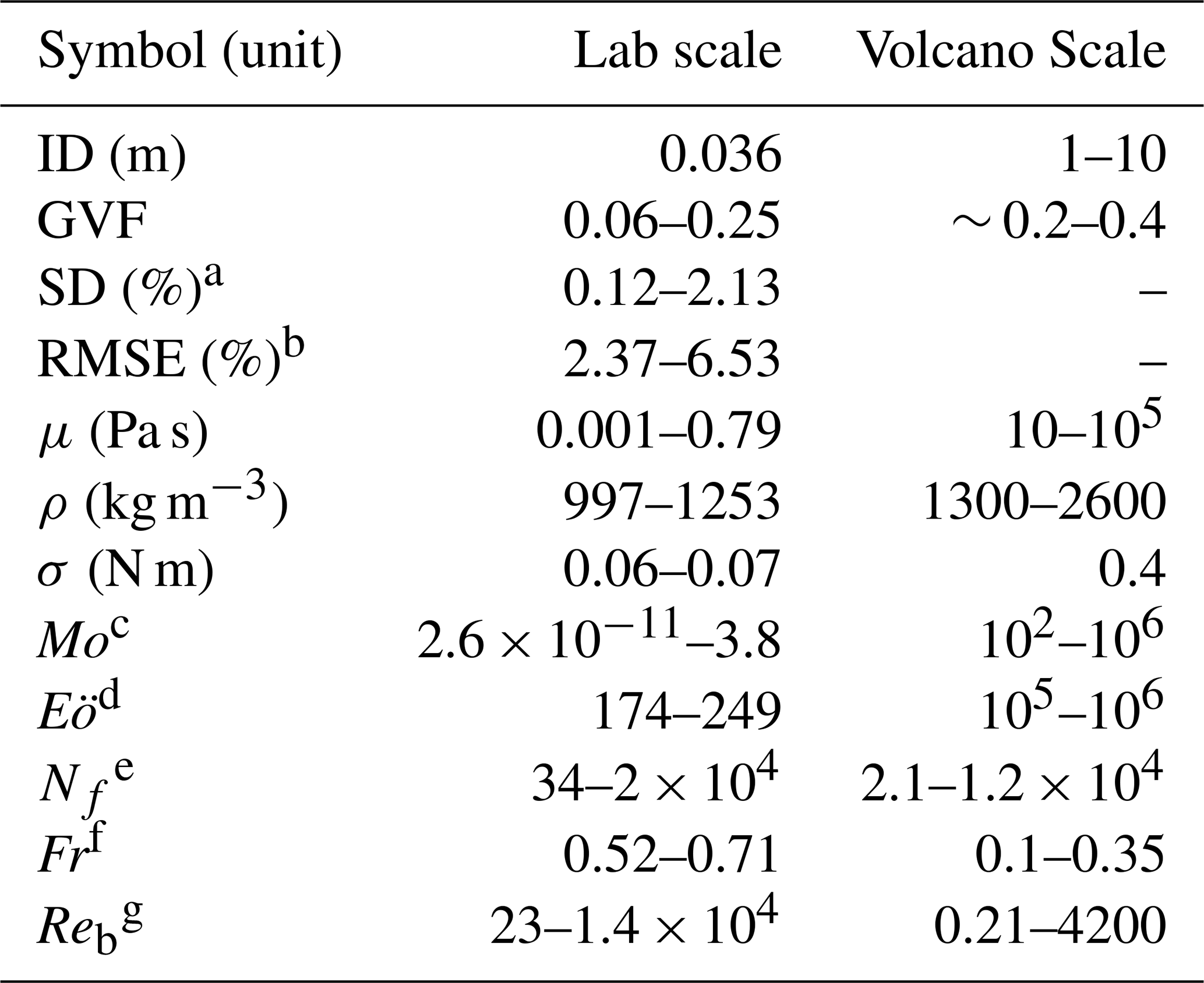
^a Standard deviation – kymograph precision.
^b Root mean squared error – kymograph precision.
^c Mo is the Morton number, Mo = $g{\mathit{\mu }}^{\mathrm{4}}/\mathit{\rho }{\mathit{\sigma }}^{\mathrm{3}}$.
^d Eö is the Eötvös number, Eö = $\mathit{\rho }g{D}^{\mathrm{2}}/\mathit{\sigma }$ (Llewellin et al., 2012) where σ is the interfacial tension between the gas and the liquid.
^e N_f is dimensionless inverse viscosity, $N_f=\frac{\mathit{\rho }}{\mathit{\mu }}\sqrt{g{D}^{\mathrm{3}}}={\left[\frac{E{\mathit{\text{ö}}}^{\mathrm{3}}}{\mathrm{Mo}}\right]}^{\mathrm{1}/\mathrm{4}}$ where g=0.981 (gravity constant).
^f Fr is dimensionless velocity, Fr = $v_{\mathrm{b}}/\sqrt{gD}$.
^g Re_b is the bubble Reynolds number, Re = $\mathit{\rho }{v}_{\mathrm{b}}D/\mathit{\mu }$.

2.2 How to generate and interpret kymographs

This method utilises the open-source image processing software ImageJ (Schneider et al., 2012). A kymograph is generated by first loading the relevant experimental footage file into ImageJ in .avi format. Audio information is discarded to conserve storage space. Then, a region of interest (ROI) line is traced on the track along which the target object moves; in this case, this is the Taylor bubble. Figure 3 demonstrates simplified schematics of the kymograph generation process using the example of a single ascending Taylor bubble. The initial line ROI positioning determines which parameters can be extracted from the kymograph. The line ROI should be drawn along the central axis of the bubble and parallel to the path of ascent for Taylor bubble and coalescence counts, Taylor bubble velocity, v_b, Taylor bubble length, L_b, length of the inter-bubble space,L_l, and liquid level, LL. For measurements of Taylor bubble diameter, D_b, and falling film thickness, λ, the line ROI should be drawn so that it is perpendicular to the path of ascent. The kymograph generation process is initiated using the in-built “image > stacks > reslice” command in ImageJ's GUI. An intensity line (a “slice”) is generated for each time point, i.e., each frame, along the line ROI and then plotted along the x-axis. This process repeats so that the intensity lines are stacked vertically along the y-axis for all frames. The resulting image is a time-space plot (the kymograph), where pixel width corresponds to distance, and pixel height corresponds to time. Real (annotated) kymograph samples generated using this method are shown in Fig. 4. Examples of unedited kymographs can be accessed through the links appended at the end of the paper.

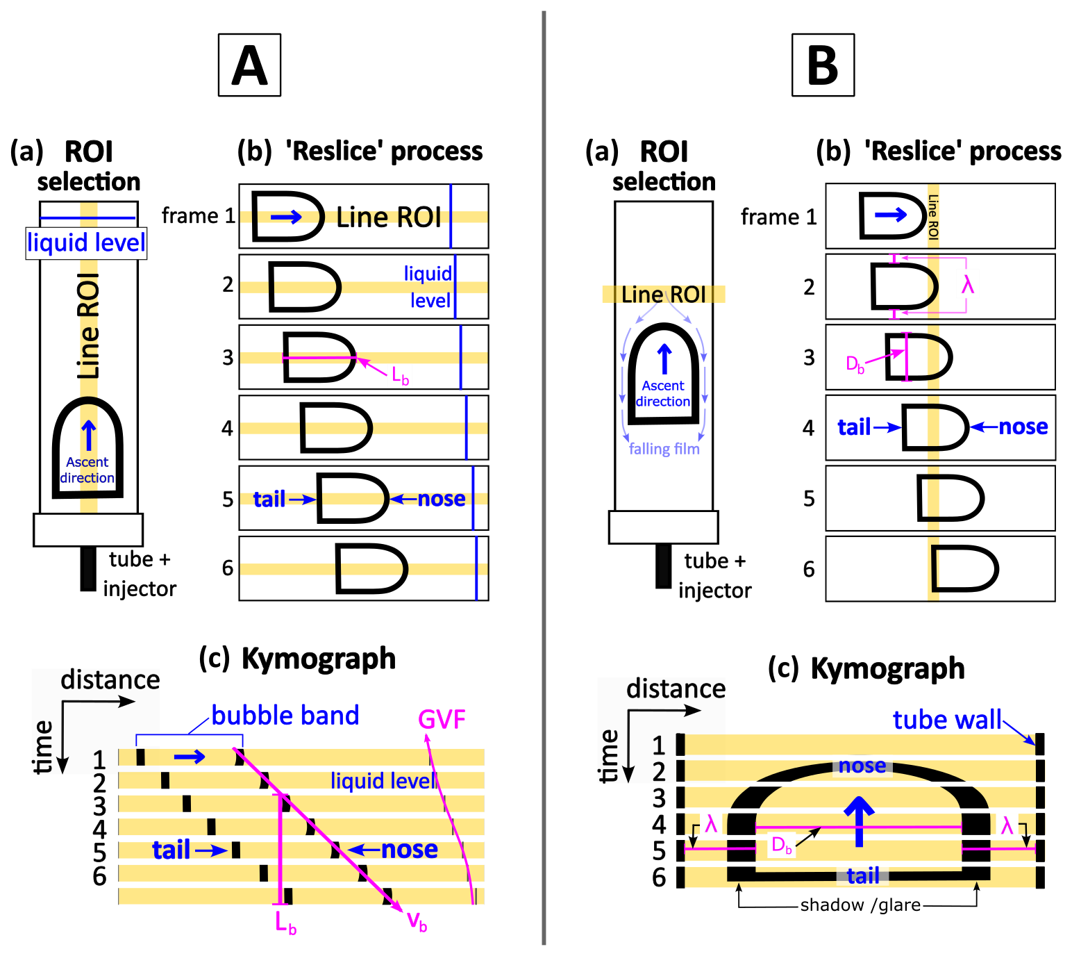
Figure 3 Simplified schematics demonstrating the kymograph generation process in imageJ using a single Taylor bubble. First, a line ROI is drawn on the imported footage, either parallel (left image – for measuring bubble velocity and length, and gas volume fraction) or perpendicular (right image – for measuring bubble diameter and falling film thickness) to the direction of ascent (a); “slices” are taken over the selected line ROI in every frame (b) and then stacked to create a single image with measurable features (c) i.e., the kymograph. Key features are shown in blue; the line ROIs required to measure/calculate key flow parameters (Taylor bubble and coalescence counts, Taylor bubble velocity, v_b, Taylor bubble length, L_b, length of the inter-bubble space, L_l, and liquid level, LL, Taylor bubble diameter, D_b, and falling film thickness, λ) on the raw footage compared to the kymographs are shown in pink.

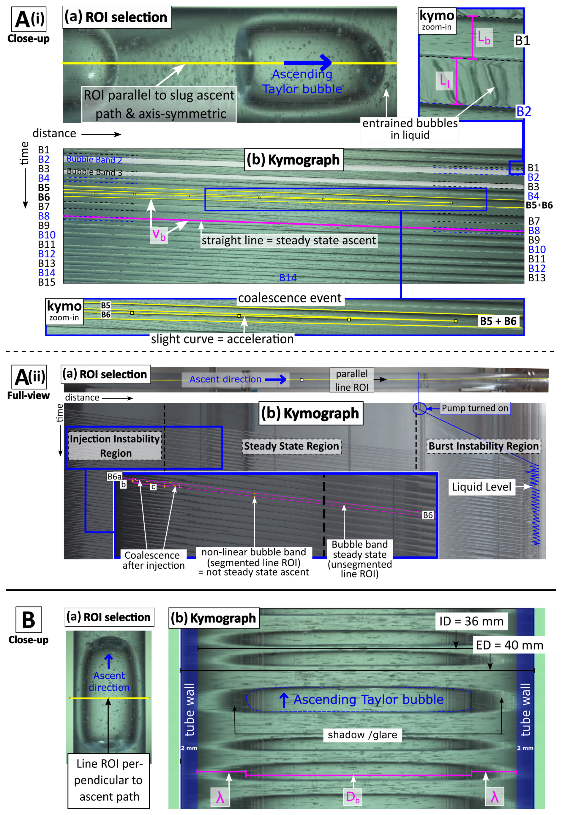
Figure 4 Annotated images of ROI selection and kymographs generated using the methods described in-text; these are labelled A or B to correspond the simplified schematics in Fig. 3; the kymographs are generated from selection ROIs parallel (A) or perpendicular (B) to the direction of bubble ascent. Key features are shown in blue; the line ROIs required to measure/calculate key flow parameters (Ai and Aii: Taylor bubble and coalescence counts, Taylor bubble velocity, v_b, Taylor bubble length, L_b, length of the inter-bubble space, L_l, and liquid level, LL; B: Taylor bubble diameter, D_b, and falling film thickness, λ) are shown in pink. Panels (Ai) and (B) are kymographs generated from close-up (100 fps) footage of a centrally located tube segment where-in the Taylor bubbles ascend in steady state. Panel (Aii) is generated from full-view (25 fps) footage that captures the full length of the tube. All the kymographs capture vertical and continuous Taylor flow (GVF = 0.25) in a liquid of 0.95 glycerol fraction.

Taylor bubble noses and tails appear on the kymographs as lines with high image contrast in the x-direction. The space in between these lines (the low-contrast region) represents the body of the Taylor bubble. We refer to these features as they appear on the kymograph as bubble bands. The spaces in between the bubble bands i.e., between the lines representing the base of a leading bubble and the nose of the next bubble ascending in the train, are the inter-bubble spaces, or liquid slugs. We refer to these features as they appear on the kymograph as liquid bands. Bubble bands are differentiated from liquid bands by the flow direction of the small (< 1 cm) entrained bubbles and how they appear on the kymograph as a result of the way they interact with the reslice line ROI (Fig. 4Ai). They can also be identified by the merging of two bubble bands, which indicates a coalescence event (Fig. 4Ai). The number of bubble bands present on the kymograph indicates the number of ascending Taylor bubbles present in the footage sample. Bubble and coalescence event counts can be extracted by simply counting these bands.

The kymographs generated from close-up footage (Fig. 4Ai and B) capture a limited (∼ 15 cm) segment of the tube, provide high resolution (captured in 1920 × 1080 pixels at 100 fps, 60 Mbps) data and are well-suited for measurements of Taylor bubble velocity, length, and diameter, liquid slug length, and falling film thickness (depending on the orientation of the selection ROI). In this case the target segment captures bubbles that have reached steady state, with the exception of low viscosity mixtures with localised turbulence. The full-view kymographs (Fig. 4Aii) capture all bubble and liquid behaviour (for the parallel selection ROI) from injection to burst: Taylor bubble velocity and length, liquid slug length, liquid level (needed for the calculation of GVF), and all coalescence events. Full-view kymographs can be divided into three regions: the injection instability region, the steady state region, and the burst instability region. The injection instability region begins at the initial injection point and ends at the approximate location along the tube where bubbles tend to enter steady state, and the steady state region begins. The start of the steady state region corresponds to the distance along the tube where Taylor bubbles are observed to stabilise, equivalent to ∼ 16D (Taitel et al., 1980), around 0.57 m along the tube. The majority of recorded coalescence occurs in the injection instability region immediately after injection. Bubble bands in this region are labelled as sub-divisions of the bubble they coalesce into upon reaching the steady state region (e.g., B6a–c in Fig. 4Aii). The burst instability region describes the approximate distance along the tube where the bubbles destabilise before burst.

2.3 Calibration, limitations, error and corrections

Detailed information on camera calibration, distortion correction, pixel-to-meter calibration, error calculation, and filtering and thresholding processes is provided in the Appendices. Pixel to world unit (m s⁻¹, m) calibrations are performed using objects in the image with a known distance e.g., the tube diameter, to determine a scale factor that is later applied to the relevant data. The clarity and readability of the generated kymographs and the data that can be extracted from them are dependent on the frame rate and resolution of the recorded footage, the FOV of the camera, the setup and lighting, and the stability of the recorded flow. Footage showing stable flow produces more coherent kymographs and thus reduced error relative to data from lower viscosity media, even at low framerates. In turbulent flows, such as in water, the larger dispersed bubbles present in the surrounding liquid and the more chaotic flow behaviour generate noisier kymographs and increased precision error. This behaviour is demonstrated in the trends observed in all the measured parameters in water as shown in Sect. 2.4–2.6; the glycerol data demonstrate strong precision between methods and less variation within the same experimental conditions because the overall flow stability is much greater than in water. Measurement precision decreases with increasing kymograph resolution because selection variability increases when pixel coverage is higher, as reflected in the data plots herein.

The precision of pixel selection by the user (“human error”) and the distortion caused by the camera lens are combined to give the root-mean-square error (RMSE). Human error was quantified as the standard deviation of repeat measurements of a single feature in millimetres (converted from pixels) for each generated kymograph i.e., based on experiment condition, camera FOV, and the initial ROI selection (parallel or perpendicular to the direction of bubble ascent). The camera has in-camera automatic distortion correction (as determined by performing checkerboard calibration) with calculated mean reprojection errors of 0.91 and 0.14 pixels, equivalent to 0.013 and 0.79 mm, for the close-up and full-view footage FOVs, respectively. Refraction at the curved boundaries along the tube cross section is found to affect all measurements taken perpendicular to the direction of bubble ascent, i.e., bubble diameter and falling film thickness measurements. A correction can be applied to the data retroactively to account for this (see Appendix D), or it can be corrected for during ROI selection as described in Sect. 2.6. Distortion along the tube length is negligible and primarily driven by the lens distortion in the camera; it is thus accounted for in the calculated error.

Image filtering and thresholding techniques including Gaussian, median, and Fourier-transform filters were applied in an attempt to enhance kymograph accuracy but ultimately failed, as they eroded critical features and reduced measurement precision. Automation attempts were also unsuccessful for similar reasons (see Appendix E). As kymography is further refined, particularly through advances in imaging and AI, its utility for the automated collection of Taylor flow parameters is likely to expand.

2.4 Velocity

The ascent velocity of volcanic Taylor bubbles (along with conduit geometry and magma viscosity) is a key control on flow stability and overpressure, and thus surface explosivity. Bubble coalescence influences eruption periodicity and repose, and is similarly modulated by magma viscosity and conduit conditions, in addition to bubble and liquid velocities. The ability to observe and measure these parameters experimentally is essential for understanding the in-conduit flow processes that drive surface explosivity and activity transitions. On a kymograph, objects moving with constant velocity appear as straight lines, where the slope of the line is directly proportional to the velocity of the moving object. The velocity of Taylor bubbles rising in steady state is determined by drawing an unsegmented line ROI along the edge of the relevant bubble band on the kymograph, then utilising the “Velocity Measurement Tool” (VMT) macro for imageJ (https://github.com/avmann/Velocity_Measurement_Tool_askScale/blob/main/Velocity_Measurement_Tool_askScale_0.3.2.ijm, last access: 25 July 2025) to measure the velocity of the line segment in pixels, and scaling to the appropriate unit (m s⁻¹) using calibrated measurements. Taylor bubbles ascending in non-steady state appear on the kymographs as non-linear bands, such as during coalescence (Fig. 4Ai) or in turbulent flow. The oscillating movement of Taylor bubbles ascending in a turbulent regime appear as irregular bubble bands which expand and contract in the y-direction on the kymograph. The acceleration of the trailing bubble is illustrated on the kymograph as a slight curvature in the corresponding bubble band as it is captured into the leading bubble wake, up to the point of coalescence. This can also be measured using the VMT with a segmented line instead, so that velocity values are calculated for each line segment.

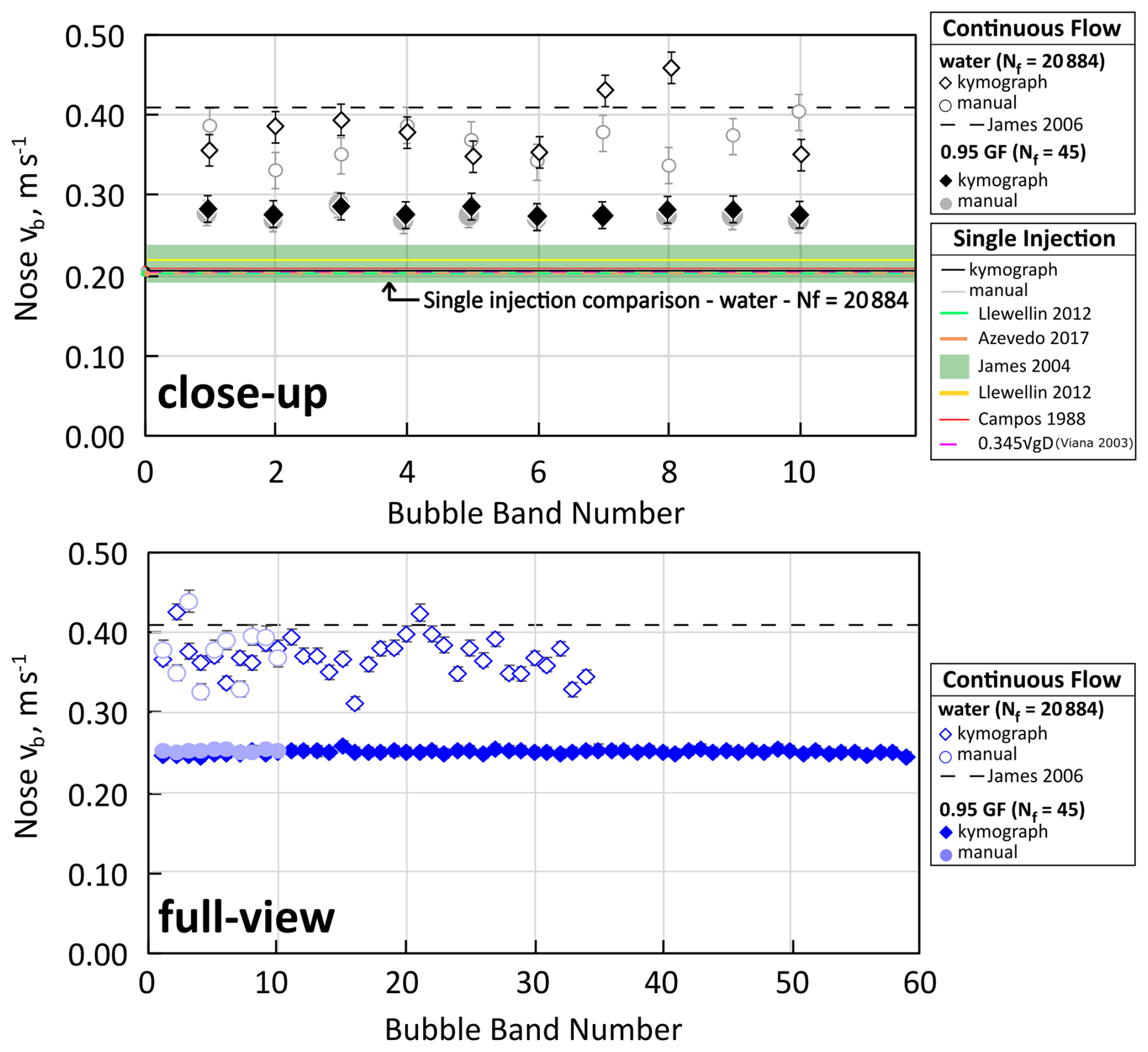
Figure 5 Kymograph ascent velocity data compared to results from manual measurements for continuous Taylor flow and a single isolated Taylor bubble injection in identical conditions for close-up and full-view FOVs. The close-up FOV plot compares kymograph measurements from ∼ 5 s of footage to manual measurements and data from the literature (de Azevedo et al., 2017; Campos and Guedes De Carvalho, 1988; James et al., 2004, 2006; Llewellin et al., 2012) under similar experimental conditions (0.035 m < D < 0.04 m) in water and to the theoretical prediction from Viana et al. (2003). Note that many of these overlap on the plot. The full-view FOV plot shows measurements for ∼ 10–30 s of footage under the same conditions. The full-view FOV demonstrates data from ∼ 30 s of footage. Calculated error is shown for the kymograph and manual measurements. Error bars that are smaller than the data markers are not visible on the plot.

Figure 5 presents Taylor bubble velocity data from 5–30 s of experiment footage where Taylor bubbles ascend in steady state in water or a solution with 0.95 glycerol fraction in continuous flow (GVF = 0.25). Results compare well to a sample of 10 point-to-point measurements from the raw footage i.e., where average velocity is calculated from the time taken for the Taylor bubbles to cover a known distance, and data from existing literature. We refer to the point-to-point measurements as “manual measurements” herein. The kymograph data show good agreement to the manual measurements in all cases, especially where flow conditions are more stable. Data from existing literature for similar experimental conditions under continuous flow are scarce, though there is good agreement with data from (James et al., 2006). There are, however, many publications exploring a broad range of isolated Taylor bubble ascent parameters (see Calleja and Pering, 2023; Morgado et al., 2016, reviews and references therein) to which we compare our results. Manual and kymograph measurements were performed for isolated Taylor bubble injections only for comparison to studies where D=0.036 ± 5 mm and in water. The processed data from the kymographs show good agreement with the studies, within a margin of 0.03 m s⁻¹ or 12 %. We also compare our results to the theoretical prediction of the ascent velocity of volcanic slugs, v_sl, assuming isolated Taylor bubble ascent within a stagnant Newtonian fluid in a vertical tube:

$$\begin{array}{}\text{(1)}& v_{\mathrm{sl}}=\mathrm{0.345}\sqrt{gD}\end{array}$$

where g is the gravitational constant and D is the internal tube diameter (Viana et al., 2003). Measurements in water show greater variation both within the same dataset and between the different methods because of the natural instabilities and turbulence that occurs in this media. Data form stable ascent conditions i.e., the higher-viscosity glycerol data show very little variation between the kymograph and manual measurements. This highlights the efficacy of kymography in this use case, especially in efficiently processing large bubble samples.

2.5 Length

Taylor bubble length influences the volume of gas released at burst, and longer Taylor bubbles are linked to increased overpressure and stronger eruptions at burst (Del Bello et al., 2012; Suckale et al., 2010). Understanding the in-conduit controls on Taylor bubble length during ascent via flow experiments improves our understanding of in-conduit gas-liquid dynamics and eruption behaviour at true scale. On a kymograph, the height of the bubble bands and the liquid bands correspond to the length of the Taylor bubbles and the inter-bubble spaces (or liquid slugs), respectively. Taylor bubble length is calculated by first drawing a vertical line ROI which starts at the band line that corresponds to the bubble nose, and ends on the band line that corresponds to the bubble base (Fig. 4Ai) and extracting its time coordinates, then multiplying the converted y-coordinates in seconds by the known ascent velocity as follows:

$$\begin{array}{}\text{(2)}& L_{\mathrm{b}}=v_{\mathrm{b}}\left(t_{\mathrm{base}}-t_{\mathrm{nose}}\right)\end{array}$$

where t_base and t_nose are the time coordinates, in seconds, which correspond to each point of the vertical line ROI. The length of the inter-bubble space is calculated using an almost identical method where the vertical line ROI is instead positioned to cover the liquid band and the following equation is used:

$$\begin{array}{}\text{(3)}& L_{\mathrm{b}}=v_{\mathrm{b}}\left(t_{\mathrm{nose}}-t_{\mathrm{base}}\right)\end{array}$$

where v_b now refers to the nose ascent velocity of the bubble rising below the inter-bubble space within the train. Figure 6 shows Taylor bubble length data for a sample of 10 bubbles ascending in steady state in continuous flow (GVF = 0.25) compared to manual measurements in identical conditions. Taylor bubble length varies in all cases due to both the liquid properties and the coalescence rates, as expected for continuous flow. The greatest difference between the manual and kymograph measurements occurs in water because the low-viscosity-driven instabilities in the flow generate lower resolution kymographs and thus increased precision error, as discussed in Sect. 2.3. The manual and kymograph measurements are shown to agree well where flow conditions are stable.

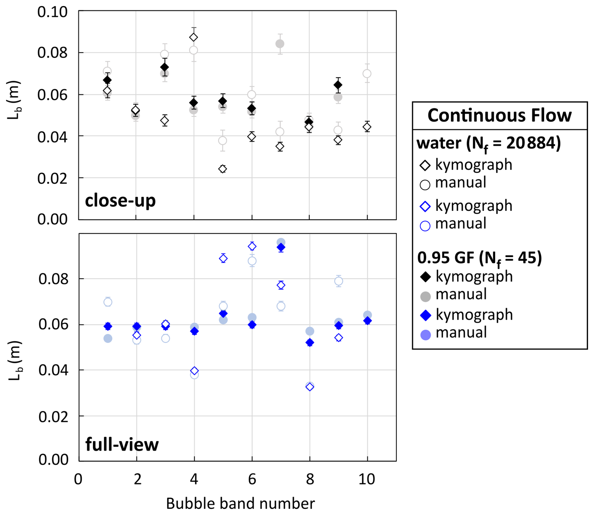
Figure 6 Kymograph Taylor bubble length data compared to results from manual measurements for continuous Taylor flow. Kymograph data are missing from bubble band numbers 7 and 10 on the close-up plot because the velocity data required to calculate length was unavailable due to coalescence, or because the end of the sample was reached, respectively.

2.6 Falling film thickness and bubble diameter

The falling film refers to the thin layer of liquid flowing downwards along the boundary between the Taylor bubble and the tube walls (Llewellin et al., 2012). The thickness of the falling film has implications for bubble stability, shape, velocity, wake behaviour and coalescence dynamics. In a volcanic conduit, the thickness of the falling magma film surrounding Taylor bubbles influences the development of overpressure and thus eruption explosivity (Del Bello et al., 2012). To measure bubble diameter and falling film thickness, the kymograph must be generated from the close-up FOV footage and using a line ROI that is perpendicular to the bubble ascent path. The resulting kymograph provides a stretched view of the target bubbles and the features needed for measurement (Fig. 4B). Differentiation of the bubble boundaries from the regions of shadow or contrast caused by the refraction of light through the tube and the liquid is crucial for accurate measurements. Misidentification of the bubble boundaries leads to underestimating falling film thickness, and overestimating bubble diameter beyond the known internal diameter of the tube. By using the known tube dimensions, it is possible to accurately identify the bubble boundaries. Once these features are correctly identified, bubble diameter and falling film thickness are measured using horizontal line ROIs as shown previously in Fig. 4B, then converting to the appropriate unit. This method of ROI selection negates the need to mathematically correct the data for the effects of refraction at the curved boundaries along the tube cross-section, as evidenced by agreement with experimental and theoretical data from the literature. An alternative approach for measuring bubble diameter and falling film thickness which requires post-processing corrections to account for image distortion by diffraction is available in Appendix D.

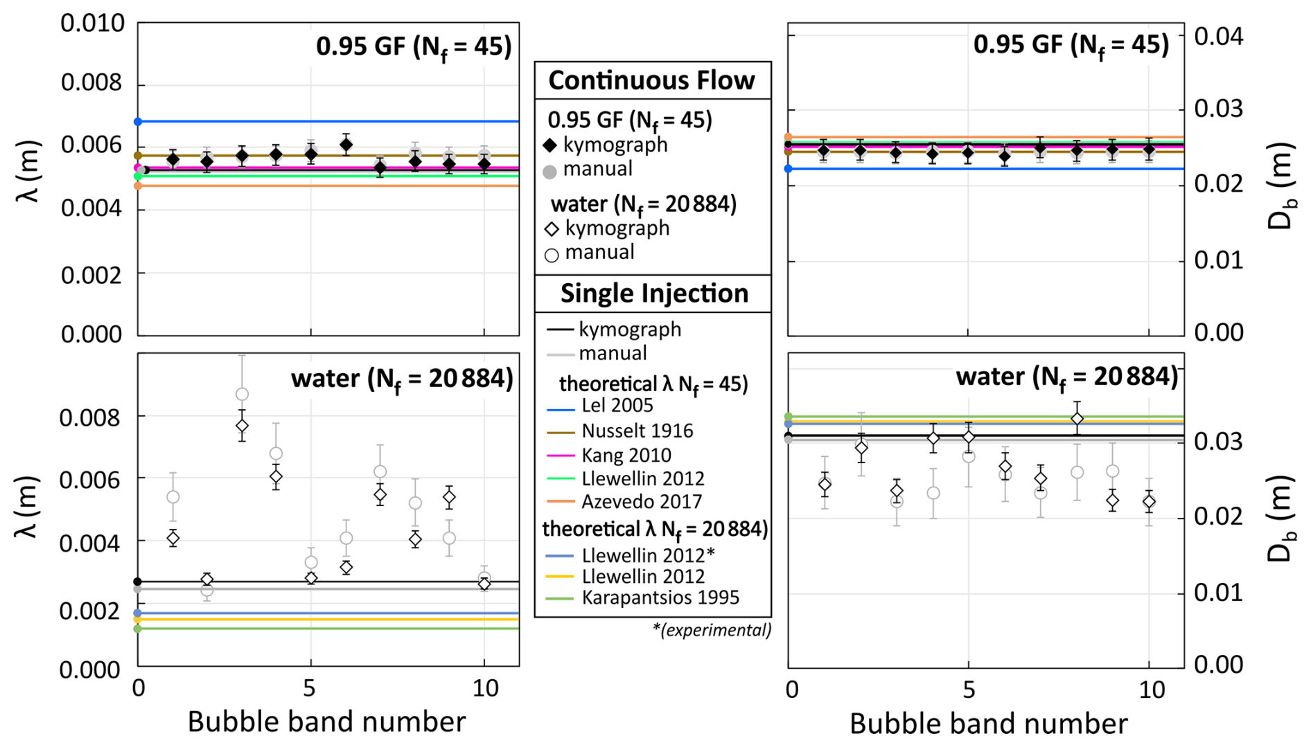
Figure 7 Taylor bubble diameter and falling film thickness. Kymograph data is compared to results from manual measurements for continuous Taylor flow in identical conditions. Single injection kymograph and manual data are also compared to estimates from empirical correlations in the literature (de Azevedo et al., 2017; Kang et al., 2010; Karapantsios and Karabelast, 1995; Lel et al., 2005; Llewellin et al., 2012; Nusselt, 1916). Calculated error is shown for the kymograph and manual measurements.

There are several empirical correlations in the literature that estimate dimensionless film thickness, λ^′, as a function of Re or N_f, that are valid for isolated Taylor bubble ascent under our experimental conditions (de Azevedo et al., 2017; Karapantsios and Karabelast, 1995; Lel et al., 2005; Llewellin et al., 2012). The theoretical λ^′ for each correlation was calculated and then used to determine predicted λ:

$$\begin{array}{}\text{(4)}& \mathit{\lambda }={\mathit{\lambda }}^{\prime }r\end{array}$$

as rearranged from Llewellin et al. (2012). Under the assumption of an axis-symmetric laminar falling film, the predicted film thickness can be used to calculate theoretical bubble diameter for the same experimental conditions:

$$\begin{array}{}\text{(5)}& D_{\mathrm{b}}=D-\mathrm{2}\mathit{\lambda }\end{array}$$

The plots in Fig. 7 demonstrate good agreement between the kymograph and manual measurements of diameter and falling film thickness, and also between the kymograph measurements with the available theoretical and experimental data for the diameter and falling film thickness of isolated Taylor bubble ascent. Where flow is stable, the single injection predictions agree well with the kymograph data for continuous Taylor flow. This is not always the case for unstable flow, where film thickness is underpredicted by the literature correlations compared to both manual and kymograph single injection measurements.

2.7 Gas volume fraction

In gas-rich basaltic systems, the gas volume fraction (GVF) within the conduit plays a fundamental role in modulating the style, periodicity, and intensity of eruptive activity. GVF serves as both a diagnostic parameter for in-conduit flow conditions and a first-order control on explosivity and surface eruption dynamics. The critical GVF required for stable slug formation and ascent defines the onset conditions for Strombolian activity, where the coupling between the Taylor bubble and the overlying magma determines whether sufficient overpressure can accumulate to generate an explosion at the surface. As such, it is vital that we are able to determine the GVF within the experimental system to ensure volcanic scalability (Table 2).

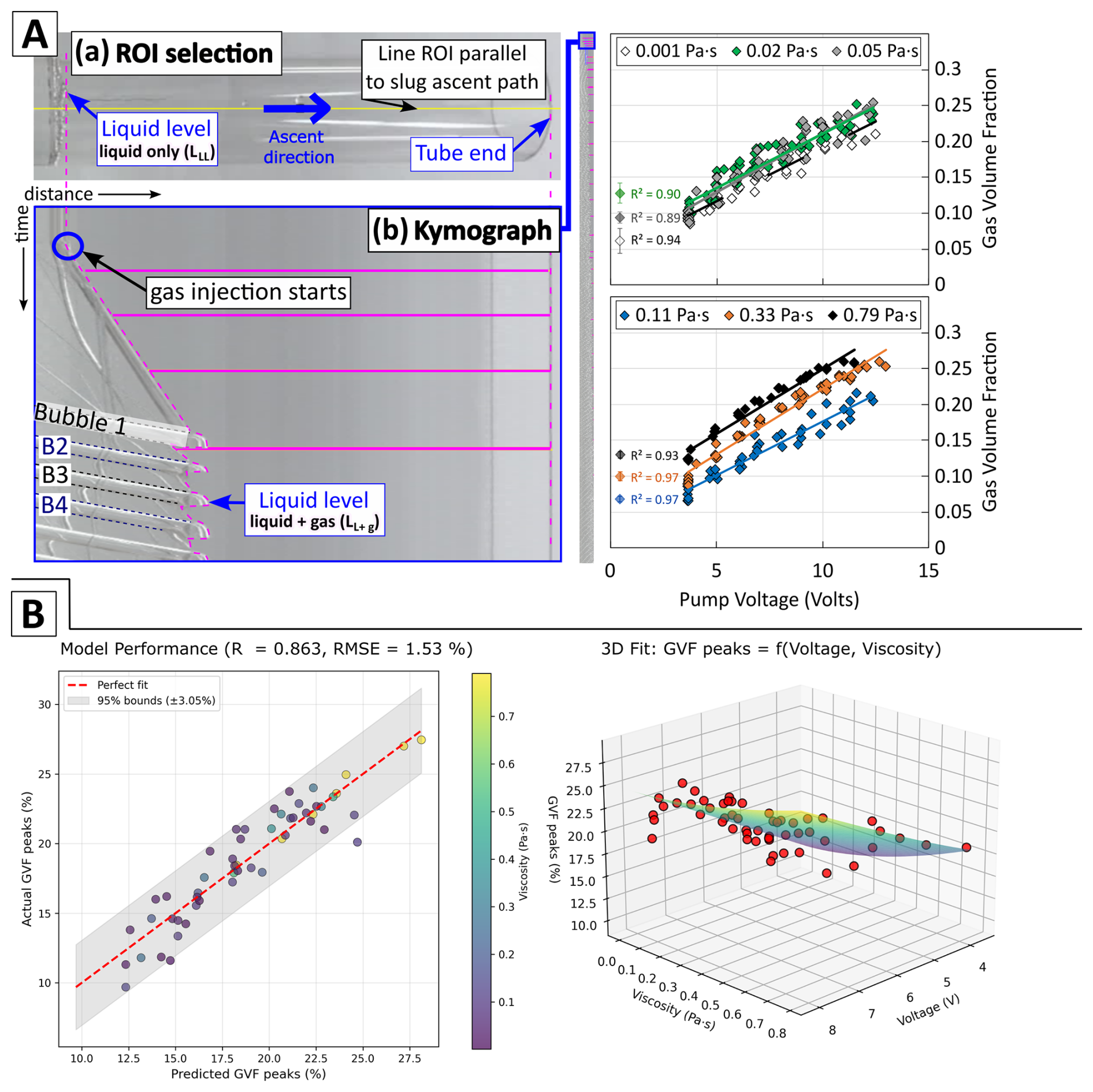
Figure 8 Liquid level and gas volume fraction (GVF). Panel (A) shows close-up view of the ROI selection (a, b) a small segment (annotated) of the entire kymograph generated to demonstrate measurements of liquid level fluctuations as pump input voltage is varied; these are used to calculate the gas volume fraction within the experimental system. The kymograph captures vertical and continuous Taylor flow (∼ 4–12 V or GVF = 0.05–0.25) in a liquid of 0.95 glycerol fraction. The plots show the full GVF capability range of the pump (note the line for the 0.02 Pa s fluid overlaps the line for the 0.05 Pa s fluid and that error bars for each dataset are displayed next to the corresponding r-squared value). Panel (B) demonstrates the model performance (left) and 3D fit based on the model equation: ${\mathrm{GVF}}_{\mathrm{peaks}}=\mathrm{16.465}\cdot V^{-\mathrm{0.491}}\cdot {\mathit{\mu }}^{\mathrm{1.668}}+\mathrm{2.789}\cdot V+\mathrm{1.884}$.

Liquid level fluctuations can be quantified on a kymograph to calculate the GVF within an experimental system, and to determine the full gas injection capability of a pump (Fig. 8). To measure liquid level fluctuations throughout an experiment run, the line ROI used to generate the kymograph must pass through the end of the tube. Once generated, the tube end appears on the kymograph as a vertical line. Numerous measurement ROIs can then be drawn to span the distance between the liquid level line and line representing the top of the tube. GVF is calculated by extracting the time coordinates and line length in pixels, performing appropriate unit conversions, and then inputting the values into the following equations:

$$\begin{array}{}\text{(6)}& {\displaystyle }{L}_{\mathrm{g}}=L_{\mathrm{L}+\mathrm{g}}-L_{\mathrm{LL}}\text{(7)}& {\displaystyle }{V}_{\mathrm{L}+\mathrm{g}}=\mathit{\pi }{r}^{\mathrm{2}}{L}_{\mathrm{L}+\mathrm{g}}\text{(8)}& {\displaystyle }{V}_{\mathrm{g}}=\mathit{\pi }{r}^{\mathrm{2}}{L}_{\mathrm{g}}\text{(9)}& {\displaystyle }\mathrm{GVF}=\left({\displaystyle \frac{V_{\mathrm{g}}}{V_{\mathrm{L}+\mathrm{g}}}}\right)\end{array}$$

where L_LL is the length of the liquid level in the tube without bubbles, i.e., before the pump is active, L_L+g is the fluctuating liquid level in the tube in meters during gas injection, L_g is the length in the tube in meters that is made up of gas only, V_L+g is the volume of liquid and gas in the tube during the gas injection process in meters cubed, V_g is the volume of gas only in meters cubed, and ris the internal radius of the tube in meters. We demonstrate the use of this method to determine the injection capability of a Delaman^® 12 V DC miniature diaphragm pump for a range of liquid viscosities in Fig. 8A, then show how these data be can used to develop a model that predicts GVF within an experimental system where pump voltage and liquid viscosity are known Fig. 8B. Gas volume fraction is shown to increase with increasing pump input voltage as expected. The model predicts GVF peaks with an R² of 0.863 and a root mean square error of 1.5 %; individual predictions have uncertainty of approximately ±3.1 % at the 95 % confidence level. Full details are available in Appendix F.

3 Concluding remarks

Taylor bubbles are recognized in volcanology as key drivers of Strombolian explosions, a prevalent form of basaltic sub-aerial volcanism. The accurate measurement and analysis of their flow parameters experimentally is essential to our understanding of subsurface Taylor bubble ascent dynamics at volcanic scales, and thus the potential to predict changing surface eruptive activity. This study demonstrates, for the first time, the application of kymography as a tool for measuring Taylor bubble flow parameters in transparent cylindrical pipes in the context of deepening our understanding of bubble-driven volcanic eruption mechanisms. Key flow parameters can be characterised, including bubble and coalescence event counts, bubble rise velocity, bubble length, liquid length, bubble diameter, falling film thickness, and gas volume fraction. In a volcanic conduit, these parameters have important implications for flow stability, interaction dynamics, overpressure development, and the volume of gas released at burst, which ultimately aids our ability to understand and predict volcanic eruption style, periodicity, repose, and explosivity level. In transparent cylindrical tubes, we show kymography to provide precise measurements even under turbulent flow conditions and at low resolutions (25 fps). Measurement precision is influenced by factors such as frame rate, camera field of view, lighting, flow stability, and the rectilinearity of the lens used for image acquisition. The accuracy of this method, validated through agreement with experimental and theoretical data from similar studies (de Azevedo et al., 2017; Campos and Guedes De Carvalho, 1988; James et al., 2004, 2006; Kang et al., 2010; Karapantsios and Karabelast, 1995; Llewellin et al., 2012; Nusselt, 1916; Viana et al., 2003), establishes kymography as a simple and effective tool for capturing detailed Taylor-bubble flow data experimentally. This method utilises an accessible and cost-effective experimental setup and open-source software, and is well-suited for the investigation of bubbles ascending with axisymmetric ascent paths in transparent media. In the context of Taylor bubble-driven volcanism, kymography is a powerful open-access tool that can facilitate efficient interpretation of analogue experiments that vitally provide a rigorous first order understanding of the governing flow processes in volcanic conduits.

Appendix A: Camera information

Table A1 Camera model and shoot settings.

Appendix B: Distortion by the camera lens

Camera calibration was performed prior to all experiments to assess the need for distortion correction and to evaluate the in-built correction capabilities of the cameras. Each camera view (close-up and full-view) was calibrated separately using a checkerboard (rectangular with a clear white border and fixed to a rigid surface) pattern covering ≥ 20 % of the field of view (FOV), with different checkerboard sizes selected to suit each view. The calibration workflow followed standard practices (Heikkilä and Silvén, 1997; Zhang, 2008): the camera was fixed on a tripod and manually focused on the tube, and the checkerboard was moved through the FOV at varied angles and orientations to maximise lens distortion coverage, particularly near image edges. Between 10–20 images were extracted from each set of recordings (182 and 400 frames for the close-up and full-view FOVs, respectively) and imported into the MATLAB Single Camera Calibrator App (https://uk.mathworks.com/help/vision/ug/using-the-single-camera-calibrator-app.html#responsive_offcanvas, last access: 25 July 2025). This tool estimates intrinsic and extrinsic parameters via checkerboard corner detection and reports calibration quality through reprojection error, with < 1 pixel generally considered acceptable. Images with high errors were excluded to ensure geometric consistency across the dataset, and calibration accuracy was validated by assessing undistorted image previews. Both camera FOVs yielded mean reprojection errors < 1 pixel, indicating negligible distortion (Zhang, 2008) and confirming that retrospective correction was unnecessary. However, these error values were incorporated into subsequent uncertainty analyses for kymograph-derived measurements.

Appendix C: Error

We use the term “human error” in this context to specifically refer to the variance between measurements from small discrepancies in pixel selection by the user that occur during measurement ROI selections. This was quantified for each kymograph i.e., per liquid viscosity, FOV, and initial ROI selection, by repeatedly measuring a sample of the same features on each kymograph for a total of 180 measurements then calculating the standard deviation of each measurement set (in m or mm as relevant). This is combined with the relevant camera distortion error (depending on the camera settings and FOV; in mm) using the root mean squares error (RMSE) method to give the error bars that are applied to all the data presented in the main text. RSME was calculated using the standard equation:

$$\begin{array}{}\text{(C1)}& \mathrm{RMSE}=\sqrt{{\displaystyle \frac{\mathrm{1}}{n}}\sum _{i=\mathrm{1}}^n{e}_i^{\mathrm{2}}}\end{array}$$

where e_i represents the individual error values, including distortion and precision error, expressed as percentages. n is the number of error values considered (in this case, n = 2). The summation $\sum _{i=\mathrm{1}}^n{e}_i^{\mathrm{2}}$ denotes the sum of the squares of the individual errors.

For this specific calculation, the error values e₁ and e₂ correspond to the distortion error and the precision error, respectively.

Appendix D: Refraction corrections

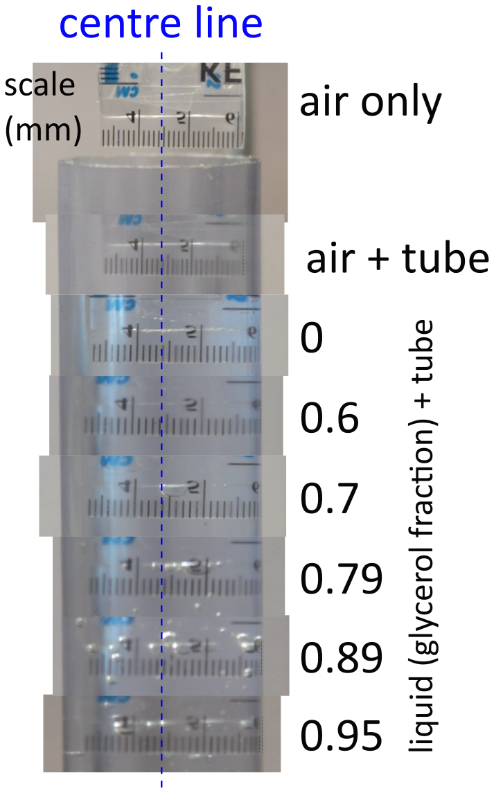
D1 Experimental quantification of distortion

To quantify distortion caused by refraction through the tube wall and liquids along the boundaries of the tube cross-section, we imaged a ruler in air, in the empty tube, and in the tube filled with each liquid Fig. D1. A web plot digitizer was then used to establish a known scale based on the tube radius (centre line to tube edge = 20 mm) then determine the actual and apparent radial distances starting from the centreline towards the edges. We found that pixel scale varies with increasing distance from the centreline of the tube. This has particular implications for measurements taken across the tube diameter i.e., falling film thickness and bubble diameter.

Figure D1 Illustration of imaging used to quantify distortion along the tube cross-section.

D2 Model methods

D2.1 Optical system and ray tracing

To consider refraction at the tube-glass interface where imaged rays are not orthogonal to the surfaces, we developed a ray-tracing model to calculate optical distortion in cylindrical PVC tubes filled with glycerol-water mixtures using Snell's law. The tube geometry consisted of an inner radius r_inner=18 mm, and outer radius r_outer=20 mm, yielding a wall thickness of 2 mm.

For the optical properties, we used the refractive indices of n_air=1.000, n_water=1.333, n_glycerol=1.474 and n_pvc=1.540. The refractive index of the glycerol-water mixtures was calculated using a linear mixing rule:

$$\begin{array}{}\text{(D1)}& n_{\mathrm{fluid}}=n_{\mathrm{water}}\left(\mathrm{1}-f_{\mathrm{g}}\right)+n_{\mathrm{glycerol}}{f}_{\mathrm{g}}\end{array}$$

where f_g represents the glycerol volume fraction.

D2.2 Calculation of ray paths

For an object at radial position r from the tube centre, we traced rays through the system by calculating the incident angle at the inner surface:

$$\begin{array}{}\text{(D2)}& {\mathit{\theta }}_{\mathrm{incident}}=\arcsin {\displaystyle \frac{r}{r_{\mathrm{inner}}}}\end{array}$$

Applying Snell's law at the fluid-PVC interface:

$$\begin{array}{}\text{(D3)}& \sin {\mathit{\theta }}_{\mathrm{pvc}}={\displaystyle \frac{n_{\mathrm{fluid}}}{n_{\mathrm{pvc}}}}\sin {\mathit{\theta }}_{\mathrm{incident}}\end{array}$$

Calculating the path length through the tube wall:

$$\begin{array}{}\text{(D4)}& L={\displaystyle \frac{r_{\mathrm{outer}}-r_{\mathrm{inner}}}{\cos {\mathit{\theta }}_{\mathrm{pvc}}}}\end{array}$$

At the PVC-air interface, we calculated the exit angle:

$$\begin{array}{}\text{(D5)}& \sin {\mathit{\theta }}_{\mathrm{air}}={\displaystyle \frac{n_{\mathrm{pvc}}}{n_{\mathrm{air}}}}\sin {\mathit{\theta }}_{\mathrm{pvc}}\end{array}$$

Positions where sin θ_air>1 indicate total reflection, rendering the object invisible at that location.

D2.3 Apparent position model

To match experimental observations, we developed an empirical demagnification model. Minimal distortion occurs in air-filled tubes:

$$\begin{array}{}\text{(D6)}& {\mathrm{demagnification}}_{\mathrm{air}}=\mathrm{1.0}-\mathrm{0.01}{\left({\displaystyle \frac{r}{r_{\mathrm{inner}}}}\right)}^{\mathrm{2}}\end{array}$$

For liquid-filled tubes, we implemented a three-component model combining angular compression, index mismatch, and edge effects:

$$\begin{array}{}\text{(D7)}& \begin{array}{rl}{\mathrm{demagnification}}_{\mathrm{liquid}}=& {\displaystyle \frac{\sin {\mathit{\theta }}_{\mathrm{pvc}}}{\sin {\mathit{\theta }}_{\mathrm{incident}}}}\times {\displaystyle \frac{n_{\mathrm{fluid}}}{n_{\mathrm{pvc}}}}\\ & \times {\left[\mathrm{1.0}-\mathrm{0.2}\left({\displaystyle \frac{r}{r_{\mathrm{inner}}}}\right)\right]}^{\mathrm{2}}\end{array}\end{array}$$

The apparent radial position is then:

$$\begin{array}{}\text{(D8)}& {\mathrm{demagnification}}_{\mathrm{liquid}}=r\times \mathrm{demagnification}\end{array}$$

D2.4 Experimental validation

The collected experimental data were loaded with the format “XXpercent.csv” where XX indicates the relevant glycerol percentage.

D2.5 Model limitations and extrapolation

The simplified ray-tracing model predicts total internal reflection (TIR) at the PVC-air interface for radial positions beyond approximately 14 mm, where the calculated exit angle of ${\mathit{\theta }}_{\mathrm{c}}=\arcsin (\mathrm{1}/\mathrm{1.54})\approx \mathrm{42.2}$. However, the experimental data clearly shows that objects remain visible up to 17.88 mm, indicating that the single-ray approximation fails to capture the complete physics.

This discrepancy arises because the model considers only a direct ray path from object to observer, where in reality objects emit light in multiple directions. Rays travelling at different angles can successfully traverse the optical system even when the direct ray undergoes TIR. The visibility of objects near the tube edge is maintained through these alternative ray paths, though with severe optical compression.

To reconcile the theory with the experimental data as closely as possible, we applied a third-degree polynomial extrapolation using the last 30 valid data points to extend the theoretical curves from 14 to 18 mm. This approach preserves the model's accuracy in the central region while providing reasonable estimates for the edge behaviour where the single-ray approximation breaks down.

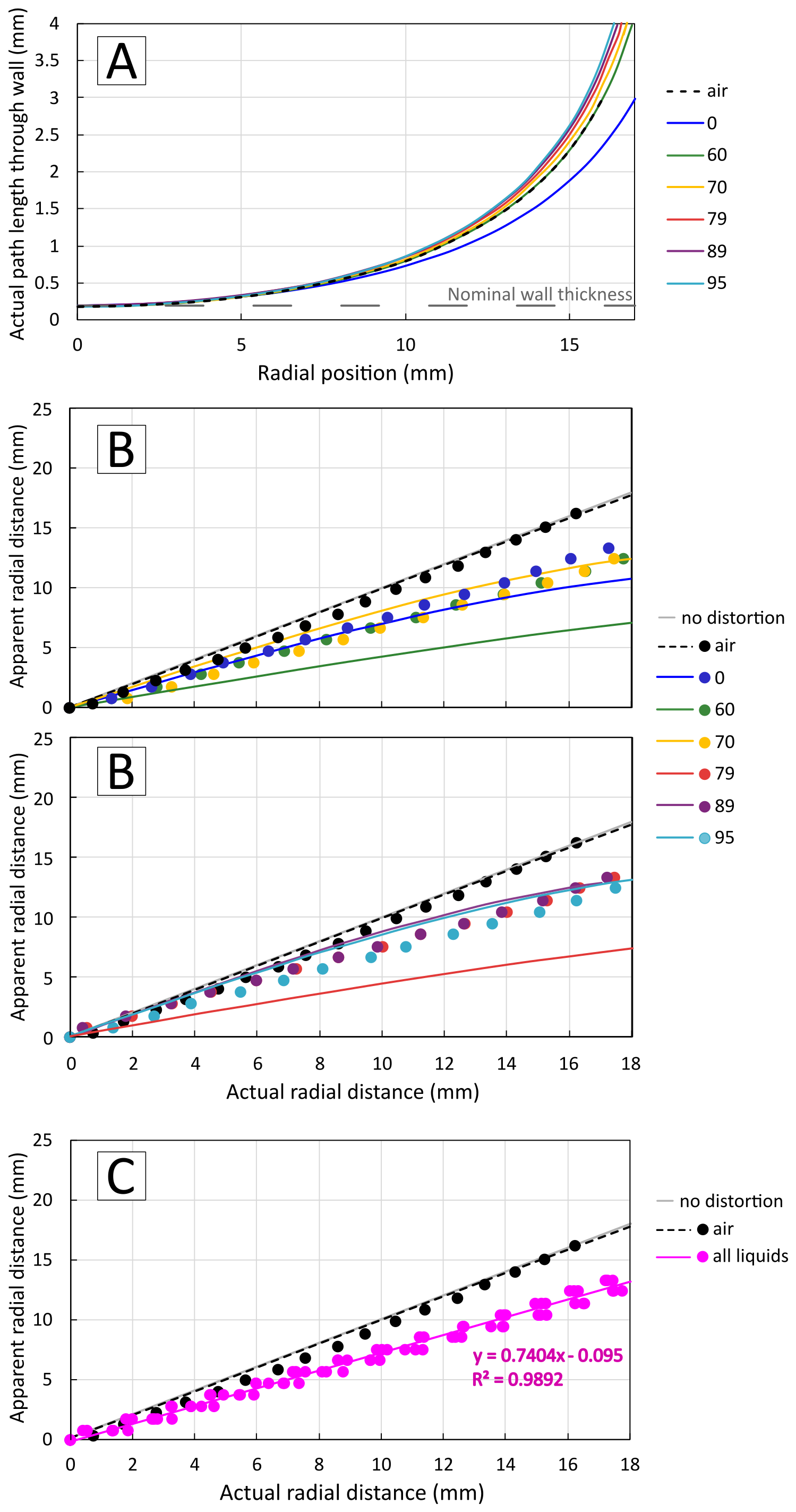
Figure D2 Panel (A) shows the calculated ray path length through the tube wall, panel (B) plots show the theoretical (solid lines) vs. experimentally quantified (markers) optical distortion (these were split into two separate plots so that overlapping data can be viewed clearly), and panel (C) shows the experimentally measured optical distortion for all liquid on a single plot, and the line equation used to apply distortion correction to the data as described in the appended text.

D2.6 Data Analysis

We compared the theoretical predictions with the experimental measurements by calculating the apparent position for each experimental datapoint and computing the mean absolute percentage error:

$$\begin{array}{}\text{(D9)}& \mathrm{Error}={\displaystyle \frac{\mathrm{1}}{N}}\sum _{i=\mathrm{1}}^N\left|{\displaystyle \frac{r_{\mathrm{apparent},\mathrm{theory}}-r_{\mathrm{apparent},\exp }}{r_{\mathrm{apparent},\exp }}}\right|\times \mathrm{100}\end{array}$$

Additionally, we generated visualisations for glycerol concentrations of 0 %, 60 %, 70 %, 79 %, 89 %, and 95 % to demonstrate the increasing optical distortion with refractive index.

Figure D2A shows the calculated ray path lengths through the tube wall, and a comparison of the predicted (Snell's law) and measured (experimental) optical distortion as it occurs with increasing radial distance from the centre point (0). The distortion through the liquids is shown to occur over a small range with a linear fit where R² = 0.99. As such, we used its line equation to apply the correction to the diameter and falling film thickness data obtained using measurement ROI method (b) described above. The code (written by ECPB) is available for download via the link at the end of the paper.

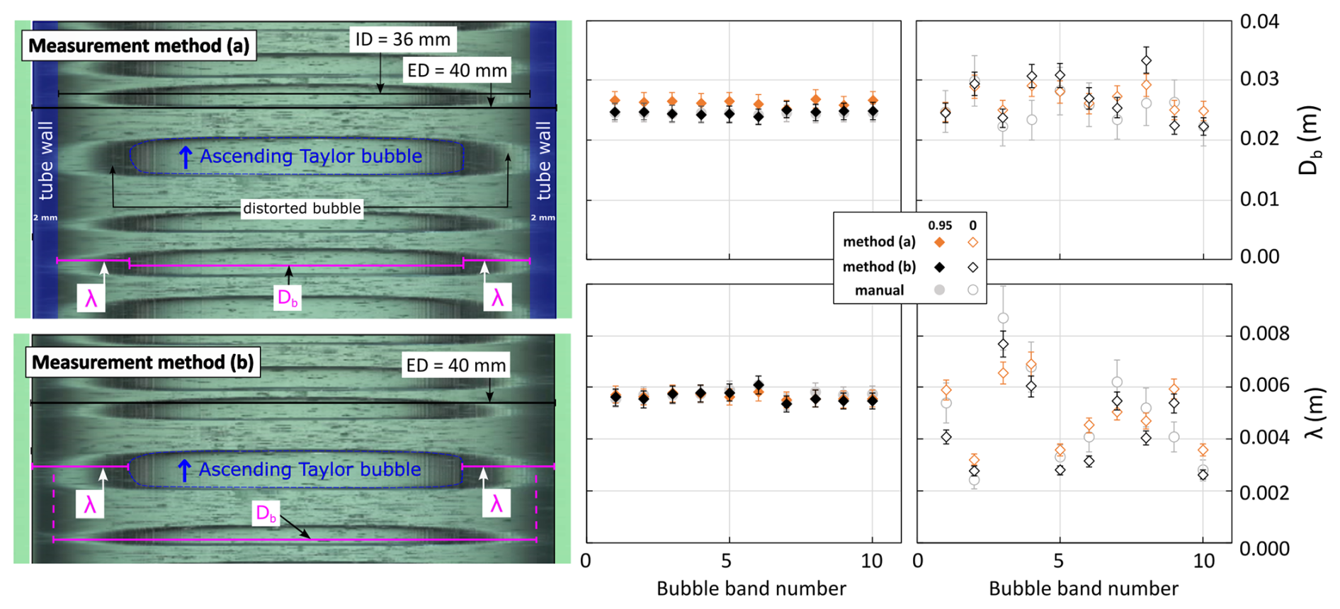
Figure D3 Annotated kymograph showing measurement ROI selections based on methods (a) – accounting for refraction during measurement ROI selection – or (b) – correcting for refraction mathematically later – as described in the Appendix text. Since the region of distortion is corrected for in method (b), it must be included in measurement ROI selections for both parameters i.e., the line ROIs overlap. The plots show the agreement between the two methods for both diameter and falling film thickness measurements.

D2.7 Results

We find that distortion can be accounted for directly on the kymographs by (a) using known measurable boundaries to identify what is and is not “bubble” or “falling film” in the kymograph i.e., by drawing the line ROI to cover the minimum bubble boundary and excluding visible distortion, or by (b) including visible regions of distortion during ROI selection then applying a correction to the data retroactively. Both parameters can be accurately measured on the kymograph using these methods (Fig. D3). The data presented in the main text utilises method (a). The correction applied to the data in method (b) utilises the line equation derived from the experimental data demonstrated in Fig. D2 in pink. Refraction-driven distortion corrections for velocity, length etc. kymographs are not needed because the measurement ROIs are drawn along the centreline of the tube parallel to the direction of ascent; distortion along the edges of the FOV are caused by the lens and captured within the calculated error. The accuracy of these methods is evidenced by the good agreement of the kymograph data with theoretical predictions or experimental data from the literature for each relevant parameter.

Appendix E: Image filtering/thresholding

Image filtering and thresholding techniques were attempted both during image pre-processing, and to the kymographs themselves, to try to remove or attenuate image noise. These include the Gaussian, median, minimum, maximum, and variance filters that are built into imageJ, and also the Fourier-transform based and ROI-width filtering algorithms that are part of imageJ kymograph plugins (DynamicKymograph: https://imagej.net/plugins/dynamic-kymograph, last access: 25 July 2025; and KymographDirect, Mangeol et al., 2016). All attempts were unsuccessful and limited overall measurement accuracy. Filtering eroded the boundaries representing key bubble and liquid features required for measurement either via a reduction in image sharpness, or by enhancing regions of glare or shadow. Automation of this technique was also unsuccessful for similar reasons. As kymography is further refined, particularly through advances in imaging and AI, its utility in volcanology is likely to expand.

Appendix F: Gas volume fraction model

To predict the gas volume fraction (GVF) in an experiment using known pump voltage and liquid viscosity values, we first characterised the behaviour of the pump and its influence on GVF. The GVF peak values (maximum GVF reached for each pump voltage and liquid viscosity) obtained using the kymograph method described in Sect. 2.7. were compiled into a CSV file (column AA in the supplied datasheet linked in the “Code and data availability” section). A custom Python script was written by ECPB to analyse this dataset and model the relationship between GVF, pump voltage, and fluid viscosity (the code is linked in the “Code and data availability” section). The script groups the dataset by unique voltage values (minimum of six unique values required to ensure adequate coverage for model fitting) then calculates the mean GVF peak, the standard deviation, the number of samples, and the average viscosity for each voltage group.

A multi-parameter nonlinear model is fitted using differential evolution optimisation to predict GVF peaks as a function of both voltage and viscosity. The functional form of the model is:

$$\begin{array}{}\text{(F1)}& {\mathrm{GVF}}_{\mathrm{peaks}}=a\cdot V^b\cdot {\mathit{\mu }}^c+d\cdot V+e\end{array}$$

Where V is the pump voltage, μ is the dynamic viscosity of the fluid, and a, b, c, d, and e are fitted model parameters: a is a scale factor, b indicates the sensitivity of GVF to pump voltage, c indicates the sensitivity of GVF to liquid viscosity, d⋅V is a linear component, and e is a constant. This model form was selected to search for the best values of a, b, c, d, ande that minimise the difference between the model's predictions and the actual GVF values we determined using the kymograph method.

Model performance was evaluated using R², root mean square error (RMSE), and residual statistics. The final model showed a high degree of explanatory power (R²=0.95), with a typical prediction uncertainty of ±3.2 % RMSE. Uncertainty intervals (e.g., 95 % confidence = ±2 × RMSE) were also reported to support predictive use in future experiments. A bootstrap resampling procedure was applied to estimate parameter uncertainties; this enabled the calculation of 95 % confidence intervals for each model coefficient. The model results are summarised below; model uncertainty bands, residual analysis plots and the distribution of residuals are displayed in Fig. F1.

Model equation:

$$\begin{array}{}\text{(F2)}& {\mathrm{GVF}}_{\mathrm{peaks}}=\mathrm{16.465}\cdot V^{-\mathrm{0.491}}\cdot {\mathit{\mu }}^{\mathrm{1.668}}+\mathrm{2.789}\cdot V+\mathrm{1.884}\end{array}$$

With R² = 0.863, the error to report for GVF peaks predictions is:

• RMSE = 1.53 % (root mean square error).

• For individual predictions: ±3.1 % at 95 % confidence level.

• confidence level.

This means that for any given (μ, V) combination, we can expect:

• 68 % of predictions to be within ±1.5 % of the true value.

• 95 % of predictions to be within ±3.1 % of the true value.

• 99 % of predictions to be within ±3.9 % of the true value.

Figure F1 Plots showing uncertainty analysis at the 95 % confidence interval (top), and residual analysis results with the distribution of residuals (bottom left and right, respectively) from the GVF model described in the appended text.

Appendix G: Unedited kymographs

The kymographs shown in the main text are small segments of the raw kymographs that have been cut down and annotated for simplicity and clarity. A sample of unedited kymographs are available as .TIFF files linked in the “Code and data availability” section under the following filename classification: “[camera FOV]_[glycerol content]_[pump voltage]” e.g., “close-up_0.95_12V” corresponds to a kymograph generated from close-up FOV footage of bubbles ascending in 0.95 glycerol content where the pump voltage input is set to 12 V.

Appendix H: Notation

Mathematical notation and abbreviations in the order that they appear in the text

Notation	Description
GVF	Gas volume fraction
fps	Frames per second
D	Internal diameter of the tube or volcanic conduit, m
FOV	Field of view
μ	Liquid viscosity, Pa s
ρ	Liquid density, kg m−3
σ	Interfacial tension, N m−1
CV	Coefficient of variation
Fr	Froude number, dimensionless velocity
Reb	Bubble Reynolds number, dimensionless ratio of inertial to viscous forces
Eö	Eötvös number, dimensionless ratio of buoyancy to surface tension forces
Mo	Morton number, dimensionless ratio of viscosity, buoyancy, and gravity forces
Nf	Dimensionless inverse viscosity
ROI	Region of interest
vb	Taylor bubble ascent velocity, m s−1
Lb	Taylor bubble length, m
Ll	Length of the inter-bubble space, or liquid slug, m
LL	Liquid level, m
Db	Taylor bubble diameter, m
λ	Falling film thickness, m
LLL	The liquid level in the tube without bubbles, m
LL+g	The combined height of liquid and gas in the tube during gas injection, m
Lg	The height of gas only within the tube during gas injection, m
VL+g	The combined volume of liquid and gas in the tube during gas injection, m3
Vg	The volume in the tube made up of gas only, m3
r	The internal radius of the tube or conduit, m
VMT	Velocity measurement tool
tbase	The point coordinate of one end of the vertical length line ROI that overlaps the band line representing the Taylor bubble base, s
tnose	The point coordinate of one end of the vertical length line ROI that overlaps the band line representing the Taylor bubble nose, s
λ′	Dimensionless falling film thickness