Improving the Magic constant – data-based calibration of phased array radars

We present a method for improved calibration of multi-point electron density measurements from incoherent scatter radars (ISR). It is based on the well-established Flatfield correction method used in imaging and photography, where we exploit the similarity between independent measurements in separate pixels in an image sensor and multi-beam radar measurements. Applying this correction method adds to the current efforts of estimating the magic constant or system constant made for the calibration of multi-point radars, increasing data quality and usability by correcting for variable, unaccounted, and unpredictable variations in system gain. This second-level calibration is especially valuable for studies of plasma patches, irregularities, turbulence, and other research where inter-beam changes and fluctuations of electron density are of interest. The method is strictly based on electron density data measured by the individual radar and requires no external input. This is of particular interest when independent measurements of electron densities for calibration are available only in one pointing direction or not at all. A correction factor is estimated, which is subsequently used to scale the electron density measurements of a multi-beam ISR experiment run on a phased array radar such as RISR-N, RISR-C, PFISR, or the future EISCAT3D radar. This procedure could improve overall data quality if used as part of the data-processing chain for multi-beam ISRs, both for existing data and for future experiments on new multi-beam radars.

1 Introduction

The polar ionosphere is highly dynamic and contains plasma structures at a large range of scales (e.g. Kintner and Seyler, 1985; Tsunoda, 1988; Tsinober, 2009). Measuring and observing the plasma, the structuring, and their spatiotemporal evolution is necessary to understand the underlying physics. It is thus connected to the larger context of how the ionosphere is coupled to the magnetosphere and the interplanetary space around us. One of the most powerful ground-based instruments to study ionospheric plasma are incoherent scatter radars (ISRs). Currently, there are six ISRs operational and one in construction (at the time of writing) in the high-latitude region in the northern hemisphere. Three of these are dish radars located in the northern Fennoscandia region and on Svalbard, and three are phased array radars located in Resolute Bay, Canada (Bahcivan et al., 2010; Gillies et al., 2016), and Poker Flat, Alaska in North America (Kelly and Heinselman, 2009). The new, state of the art, phased array European Incoherent Scatter Radar 3D (EISCAT 3D) is currently under construction in Northern Norway (McCrea et al., 2015). In contrast to dish radars, phased array radars are capable of volumetric measurements in multiple directions simultaneously (see e.g. Lamarche and Makarevich, 2017; Semeter et al., 2009, and references therein). This capability has proved itself to be a powerful tool for studying ionospheric structures such as polar cap patches and density “irregularities” (e.g. Goodwin and Perry, 2022; Lamarche et al., 2020; Forsythe and Makarevich, 2018). Electronic beam steering is used to achieve multiple beams covering the desired field of view and the temporal resolution is limited only by the time needed to achieve an acceptable signal-to-noise ratio in each beam. Depending on the given radar system, many factors affect the quality of the signal, and careful calibrations are needed for any radar.

1.1 Calibration of phased array ISR data

ISRs transmit and receive radio waves that scatter from plasma in the terrestrial ionosphere. The power spectrum of the scattered radar signal is directly proportional to the thermal electron density fluctuations and plasma parameters can then be inferred from the observed waves and fluctuations (see e.g. Evans, 1969; Fejer and Kelley, 1980, and references therein). Various factors within a given radar system will affect these measurements and their Signal-to-Noise ratio. Consequently, calculations of the plasma parameters and any absolute measurement require calibration. To make a measurement of the absolute electron density with any ISR an independent measurement is required. In many cases, the radar itself can make a measurement of the backscatter from Langmuir waves, the so-called plasma line, providing a direct measurement of the plasma frequency and thus the electron density (e.g. Bahcivan et al., 2010; Rexer et al., 2018, Sect. 3). For RISR-N and RISR-C of the Advanced Modular Incoherent Scatter Radars (AMISR), located far north in Resolute Bay, Canada, the independent measurement of electron density is particularly challenging as the weak photoelectron fluxes in the polar cap make plasma line measurements difficult. Independent measurements of the electron density for one pointing direction can also be obtained from an ionosonde (Themens et al., 2014). An ionosonde consists of an antenna and a nearby receiver that transmit and receive pulsed radio waves that are swept through the typical ionospheric plasma frequency range (0.5–20 MHz) (see e.g. Baumjohann and Treumann, 2012; Bibl, 1998). Vertically transmitted radio waves are reflected when the transmitted frequency is equal to that of the local plasma frequency, and from the time delay of the reflected signal, the altitude of reflection of the transmitted frequency can be determined. As the plasma frequency is directly related to the plasma density, we can calculate an altitude profile of the electron density on the bottom side of the ionosphere. The measured electron density from the ISR can then be scaled to match that of the ionosonde for that pointing direction. A challenge with ionosonde measurements is that this provides an independent measurement only for one general direction and only for the bottomside ionosphere. Additionally, the direction of the source of the signal in the ionosonde can be somewhat ambiguous resulting in an uncertainty of the actual receive direction of the signal and thus which radar beam and pointing direction to scale.

This issue is more complex when the radar is operated in a multi-beam mode. The power of the received signal, and thus the electron density measurements, are dependent on the two-way gain of the antenna in the direction in which it is transmitted and received. For a phased array radar, the antenna gain is maximized in one pointing direction. All beams pointing in another direction will have a different gain, which can be determined from the antenna gain pattern (radiation pattern) if known. With the antenna gain pattern, it is then possible to calculate a scaling factor for measurements for all beams off the center of the main antenna lobe.

In the AMISR radars, the antenna gain is maximized at bore-sight (Gillies et al., 2018). The antenna gain pattern is modeled, and with an independent measurement of the electron density, a scaling factor is estimated for all beams (Lamarche, 2022). In the AMISR data products, this scaling factor is given as the “system constant” or ksys. For the EISCAT radars this constant is called the Magic constant. However, even after the most meticulous technical calibration of a multi-beam radar, estimating this constant is difficult as the system gain and antenna pattern change with time. For example, an AMISR radar or the future EISCAT 3D radar might have some antenna elements fail, or parts of the array might be covered in snow and ice affecting the radiation pattern locally. Additionally, the antenna gain pattern may vary greatly with experiment, operating temperature, aging antenna components, ground conditions, etc. These changes can affect the total system gain, and ideally this should be taken into account for every experiment separately.

1.2 Flatfield calibration in imaging vs. multi-beam radars

Flat field correction is a well-established method that has been developed and applied in imaging and image processing for decades (see e.g. Montgomery et al., 1988; Burke, 1996; Oswalt and Bond, 2013, and references therein). It addresses two problems. The first is that different pixels in a sensor can have their own zero-point, that is, the minimum value on each pixel might be different due to thermal noise, material effects, or electronic effects in the system. In imaging, this is referred to as dark-signal non-uniformity. The second is that different pixels in a single sensor might have a different response (or gain) to the same level of illumination or input. This is referred to as spatial photo response non-uniformity in image sensors (see e.g. Burke, 1996, Chap. 5). When not accounted for, non-uniformities of a sensor result in false spatial patterns in the image.

The correction for the dark signal non-uniformity can be relatively straightforward in imaging and is done by subtracting a Darkfield image or bias frame. The Darkfield image is found by averaging (to reduce noise effects) over many individual images taken with the system at “operating temperature”, without exposing the sensor to light (e.g., keeping the lens cover on, not opening the shutter). Thus, no illumination can affect the sensor, and the resulting “image” contains only the Darkfield image with its non-uniformities and internal effects of the system.

The variation in gain between pixels is traditionally corrected for by a normalization, using Flatfield images (e.g. Burke, 1996). Flatfield images are obtained by taking an image of a flat field, that is, an optically flat or uniform source of light. In Astronomy, the twilight sky is often used (e.g. Oswalt and Bond, 2013). Averaging of a number of Flatfield images gives the mean Flatfield image for the system setup. Ideally, this is done with the same system settings as for the experimental measurements and ensures that any variations in gain between pixels, also between experiments or system setups, are accounted for. The corrected image intensity at pixel (u,v) are then be calculated as:

$$\begin{array}{}\text{(1)}& {\displaystyle }{I}_{\text{corr}}(u,v)=\left(I_{\text{raw}}\right(u,v)-I_{\text{Df}}(u,v\left)\right)G(u,v),\text{(2)}& {\displaystyle }G(u,v)={\displaystyle \frac{\stackrel{\mathrm{‾}}{I_{\text{Ff}}}-\stackrel{\mathrm{‾}}{I_{\text{Df}}}}{I_{\text{Ff}}(u,v)-I_{\text{Df}}(u,v)}},\end{array}$$

where I_corr(u,v) is the corrected image, I_raw(u,v) is the raw, uncorrected image and the Darkfield and Flatfield images are indicated I_Df and I_Ff, respectively. Horizontal bars indicate the mean value over the respective image.

Phased array incoherent scatter radars and cameras are very different instruments designed for different measurements. However, they share a key aspect that allows us to adapt this method, traditionally used in imaging, to phased array ISR data analyses. Both attempt to measure their respective parameters over an area in space, using multiple detectors simultaneously. For cameras, a commonly used detector is the charged-coupled device (CCD), an area detector that is capable of measuring many points simultaneously in its field of view. A single modern CCD can commonly capture over 1000 pixels × 1000 pixels (1 MP) for one image. The multiple radar beams can be seen as the phased array radar analog of image pixels for our purpose. While modern phased array radars do not measure one million beams simultaneously, depending on the given radar mode, they can measure many tens of beams. Thus, the underlying principle of simultaneous, multi-point measurements is analogous in the two fields.

To adapt the Flatfield method to ISR measurements, we need to consider the properties of the measurements and how they are made. When estimating electron density using Thomson scatter (Evans, 1969), the ion-line power is related to electron density N_e, the ratio of electron and ion temperatures $T_{\mathrm{e}}/T_{\mathrm{i}}$, radar wavelength λ, transmit pulse length τ_p, distance to observing volume R, and transmit power P_TX. The radar antenna diffraction pattern, as well as any additional multiplicative factors, are represented with a magic constant Υ. As given by e.g., Vadas and Nicolls (2009), the equation for received power is:

$$\begin{array}{}\text{(3)}& P_{\text{RX}}={\displaystyle \frac{\mathrm{{\rm Y}}{P}_{\text{TX}}{\mathit{\tau }}_{\mathrm{p}}}{R^{\mathrm{2}}(\mathrm{1}+k^{\mathrm{2}}{\mathit{\lambda }}_{\mathrm{D}}^{\mathrm{2}})(\mathrm{1}+k^{\mathrm{2}}{\mathit{\lambda }}_{\mathrm{D}}^{\mathrm{2}}+\frac{T_{\mathrm{e}}}{T_{\mathrm{i}}})}}{N}_{\mathrm{e}},\end{array}$$

where λ_D is the Debye-length and k is the Bragg ($k=\mathrm{4}\mathit{\pi }/\mathit{\lambda }$). For a radar frequency of 440 MHz, the equation can be simplified for sufficiently large electron densities ($N_{\mathrm{e}}>\mathrm{5}\times {\mathrm{10}}^{\mathrm{10}}$ m⁻³) as follows (Vadas and Nicolls, 2009):

$$\begin{array}{}\text{(4)}& P_{\text{RX}}={\displaystyle \frac{\mathrm{{\rm Y}}{P}_{\text{TX}}{\mathit{\tau }}_{\mathrm{p}}}{R^{\mathrm{2}}(\mathrm{1}+\frac{T_{\mathrm{e}}}{T_{\mathrm{i}}})}}{N}_{\mathrm{e}}.\end{array}$$

For $N_{\mathrm{e}}>\mathrm{5}\times {\mathrm{10}}^{\mathrm{10}}$ m⁻³, determining $T_{\mathrm{e}}/T_{\mathrm{i}}$ is also to first order only depends on the shape of the ion-line, not N_e.

This allows electron density to be related to power as follows:

$$\begin{array}{}\text{(5)}& {\widehat{N}}_{\mathrm{e}}=P_{\text{RX}}\left(\mathrm{1}+{\displaystyle \frac{T_{\mathrm{e}}}{T_{\mathrm{i}}}}\right)R^{\mathrm{2}}{P}_{\text{TX}}^{-\mathrm{1}}{\mathit{\tau }}_{\mathrm{p}}^{-\mathrm{1}}{\mathrm{{\rm Y}}}^{-\mathrm{1}}G.\end{array}$$

In some cases, electron density is estimated from power only, without attempting to fit for $T_{\mathrm{e}}/T_{\mathrm{i}}$, but rather assuming it to be constant $T_{\mathrm{e}}/T_{\mathrm{i}}=\mathrm{1}$. This is referred to raw electron density, and included in AMISR data with the key NeFromPower/Ne_NoTr. Measurements that include a fitted $T_{\mathrm{e}}/T_{\mathrm{i}}$ to the ion-line is in key FittedParams/Ne. The advantage of using the NeFromPower/Ne_NoTr data product is that it is a scaled power measurement, which does not include the non-linear Debye length effects.

If the magic constant contains an error, this will result in a multiplicative factor error modeled with G in estimated electron densities. Note that G is not to be confused with the antenna gain which often uses the same symbol. The above equation is exactly the same form as Eq. (1), with $I_{\text{raw}}=P_{\text{RX}}(\mathrm{1}+T_{\mathrm{e}}/T_{\mathrm{i}})R^{\mathrm{2}}{P}_{\text{TX}}^{-\mathrm{1}}{\mathrm{{\rm Y}}}^{-\mathrm{1}}$ and I_Df=0.

In this paper, we present a relative calibration method. The objective of this method is to find a calibration for which electron density variations measured by all beams of the radar are consistent with a reference beam. In it, an attempt is made to estimate a correction factor G that is subsequently used to scale the electron density data in the same form as in Eqs. (1) and (5). The correction factor is derived from the distribution of an electron density ratio inferred from the measurements. The method only requires the electron density data from a multi-beam radar experiment, and no external measurements are necessary. One caveat is that the method is only applicable to data where $k^{\mathrm{2}}{\mathit{\lambda }}_{\mathrm{D}}^{\mathrm{2}}\approx \mathrm{0}$. The method and calculations are shown in Sect. 2. In anticipation of the EISCAT 3D radar (McCrea et al., 2015; Kero et al., 2019), we utilize data from the AMISR phased array radar system to investigate the calibration techniques described here in three examples for different experiments and seasons. These are shown in Sect. 3. A quality and error estimate calculation is presented in Sects. 4 and 5 will provide a discussion and suggestions for future multi-point radar measurements. Section 6 summarizes our conclusions.

2 Ratio distribution correction of multi-point ISR data

We calculate a ratio of electron density measurements and use the distribution of ratios to find the optimal correction factor, G_RDC. The ratio is given by

$$\begin{array}{}\text{(6)}& N_{\mathrm{e}}^{\text{ratio}}=〈{\displaystyle \frac{\stackrel{\mathrm{‾}}{N_{\mathrm{e}}^t}}{N_{\mathrm{e}}^{\text{beam}}}}〉,\end{array}$$

where $\stackrel{\mathrm{‾}}{N_{\mathrm{e}}^t}$ is the mean electron density of all beams at a timestep t ([1 × number-of-beams] – array), while $N_{\mathrm{e}}^{\text{beam}}$ is the electron density measurement in a particular beam, and the 〈⋯〉 denotes averaging over at all timesteps of an experiment ([1 × number-of-timesteps] – array). The $N_{\mathrm{e}}^{\text{ratio}}$ thus gives the ratios of the mean electron density measurement in all beams, at each time and altitude, to the electron density measurement in one beam. For every beam this gives one $N_{\mathrm{e}}^{\text{ratio}}$ for every timestep of the experiment ([1 × number-of-timesteps] – array for every beam). Hence, we obtain a distribution of the ratios for each beam. We then make a Kernel density estimate of the distribution of these ratios for each beam. An example of this is shown in Fig. 1. Here a histogram (blue) of $N_{\mathrm{e}}^{\text{ratio}}$ for Beam 27 at 250 km during the same experiment at RISR-N and RISR-C used for the example in Sect. 3. The Kernel density estimate is shown in red. The ratio at which the maximum probability density estimate is found is taken as the correction factor, G_RDC, for that beam at that altitude. This calculation is then done for all beams at the altitude of interest. For this calculation, we can either use the electron density calculated from the fit to the ISR spectra, or we can use the electron density inferred from the backscattered power of the radar signal, $N_{{\mathrm{e}}_{\mathrm{FromPower}}}$. The difference between these options is discussed in Sect. 5. In the calculations, the altitude gate is found by the nearest-neighbor method. When doing these calculations on the electron densities calculated from the fitted Autocorrelation functions, these altitude gates are approximately 20 km while when using $N_{{\mathrm{e}}_{\mathrm{FromPower}}}$ the altitude gates are approximately 3 km in the examples from AMISR data used below. The correction factor is used to scale the corresponding electron density measurement, $N_{\mathrm{e}}^{\text{org}}$, as:

$$\begin{array}{}\text{(7)}& N_{\mathrm{e}}^{\text{corr}}=N_{\mathrm{e}}^{\text{org}}{G}_{\text{RDC}}\end{array}$$

to obtain the corrected electron density, $N_{\mathrm{e}}^{\text{corr}}$.

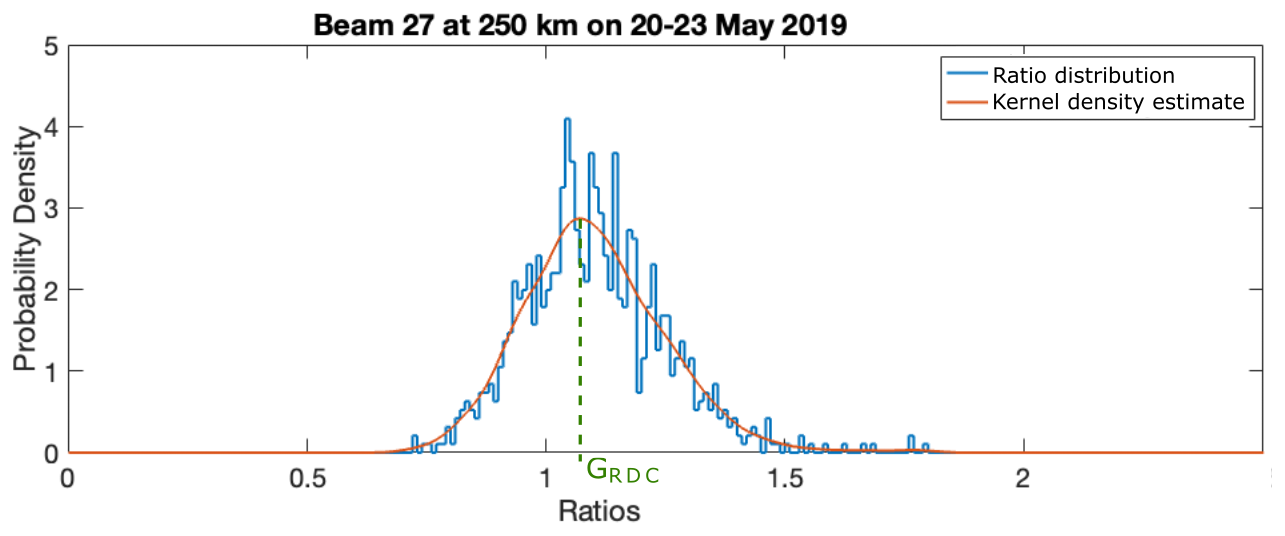
Figure 1 Kernel density estimate of the ratios between the mean of all beams at time t, and the electron density at all timesteps in beam 27 at 250 km altitude during an experiment on 20–23 May 2019. The blue line indicates the distribution of the density ratios calculated using Eq. (6). The red line shows the calculated Kernel density estimate of these ratios. The ratio, G_RDC, indicated by the green line, corresponds to the peak of the Kernel density estimate and is used as the new correction factor.

An example of how the correction factors calculated using this method can vary with beam and altitude is shown for one example in Fig. 2. Here, the electron density used for the calculations is calculated from the backscattered power of the returned signal, $N_{{\mathrm{e}}_{\mathrm{FromPower}}}$, rather than from the fit to the ISR spectra. This electron density is measured at a higher range resolution. In the calculations, the altitude gates are found by the nearest-neighbour-method. The example in Fig. 2 shows this. These correction factors are calculated here for all beams, in 3 km horizontal altitude slices during an 11-beam (22 total) experiment from 12 to 14 October 2016 at RISR-N and RISR-C (see the third example in Sect. 3).

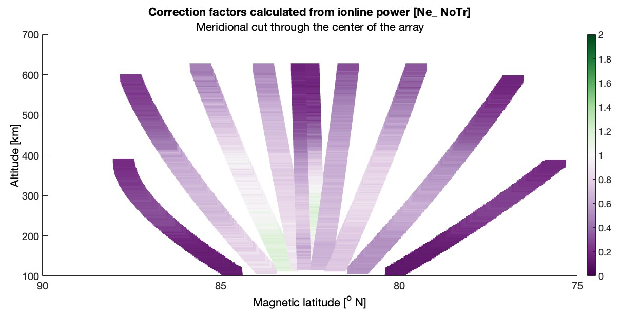
Figure 2 Calculated correction factors at all beams along the central meridian line through the arrays for the experiment running from 12 to 14 October 2016. The magnetic latitude is indicated in the x axis and the y axis indicates the altitudes. The correction factors are calculated using the raw electron density calculated from the backscattered power (Ne_ NoTr).

The figure shows all beams along a longitudinal cut at the center meridional line of both radars. It is particularly clear from this figure that the two vertical beams from the two radars are not calibrated to match in the uncorrected electron density data as they have very different correction factors. It should be noted that this difference is also explained by the large error estimate (not shown) of these two beams.

3 Examples

The results of this method are shown in the following three examples. The method presented here is applicable to any multi-point radar measurement. In anticipation of the EISCAT 3D radar (McCrea et al., 2015; Kero et al., 2019), we utilize data from the AMISR phased array radar system to investigate the calibration technique described above. Hence, we have chosen three experiments, running different radar modes with different numbers of beams from the large RISR-N and RISR-C databases. All data shown here was downloaded from the online databases and error-filtered as suggested in the AMISR user manual (Lamarche, 2022). That is, electron density measurements smaller than or the same size as the error estimate, dN_e, and data where the data quality parameters were poor, were excluded (set to Not-a-number). The error estimate and data quality parameters are normal data products provided for all RISR-N and RISR-C data. In our examples, we have used the electron density inferred from the fit to the ISR spectra, \FittedParams\Ne. Although the electron density from the backscattered power of the radar signal, \NeFromPower\Ne_NoTr, may also be used for this. To show the results of the calibration method, for each example (see Figs. 3–5), we show the uncorrected electron density for all beams at one altitude in the top panel. The beams are ordered by magnetic latitude (y axis) so that all beams from RISR-N are in the upper half, while beams from RISR-C are shown in the lower half of the panel. The plots show uncorrected densities from the experiments for the times (x axis) where both radars were running simultaneously. The bottom panel of each figure shows the densities after the Ratio distribution correction. In Fig. 5, additional white lines and white shaded areas indicate the position of the terminator at the given altitude during the experiment. As the beams in this plot are organized only by their magnetic latitude, the terminator in these plots is jagged rather than a smooth line as it would be in a polar plot. Figures 3 and 4 do not have these, as the ionosphere in the field of view of the radars was continuously sunlit during these experiments.

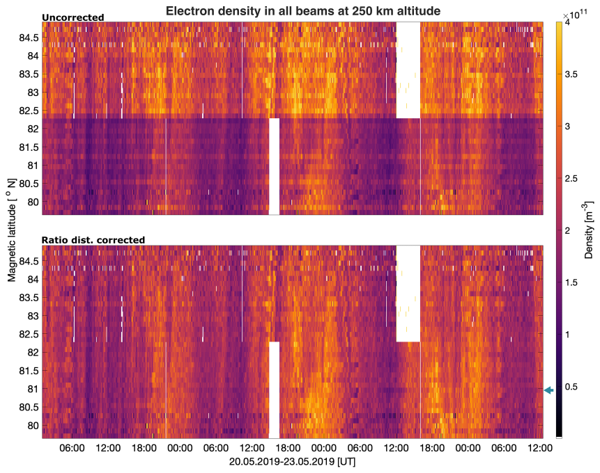
Figure 3 Electron density at 250 km altitude from 38 beams, measured at RISR-N and RISR-C in the imaginglp radar mode from 19 May 2019 22:01:09 UT to 23 May 2019 14:19:46 UT. The top panel is the uncorrected, error-filtered, electron density from the fitted ISR spectrum as downloaded from the online databases. The bottom panel shows the Ratio distribution corrected electron densities. All beams are sorted by magnetic latitude (y axis) such that RISR-N beams appear on the top half of every panel, while RISR-C beams are on the bottom half. The small blue arrow to the right, in the bottom panel indicates beam 27 used as an example in Fig. 1.

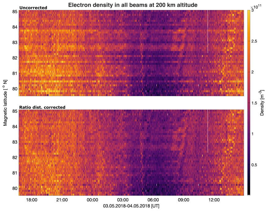
Figure 4 Electron density from the fit to the ISR spectrum at 200 km altitude from 44 beams, measured at RISR-N and RISR-C in the Convection67m radar mode, from 3 May 2018 15:55:25 UT to 4 May 2018 14:59:45 UT. The Figure is in the same format as Fig. 3.

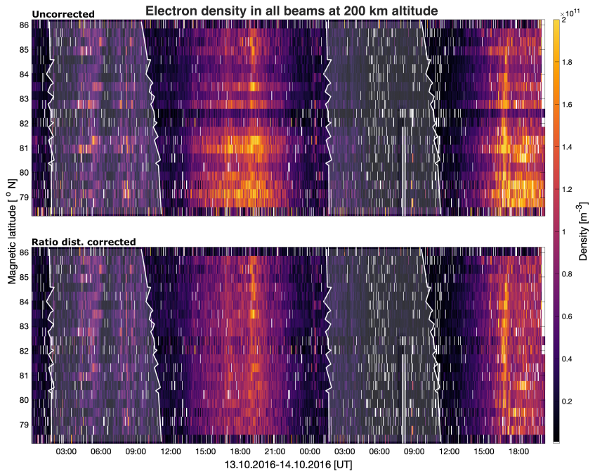
Figure 5 Electron density from the fit to the ISR spectrum at 200 km altitude, measured at RISR-N and RISR-C from 12 October 2016 21:27:07 UT to 15 October 2016 13:59:26 UT. The Figure is in the same format as Figs. 3 and 4. This Figure also shows the position of the terminator/shadow at this altitude, indicated by the white lines. The gray shaded regions in all panels indicate when the ionosphere is in darkness (shaded).

The first example is from an imaginglp experiment run from 19 May 2019 22:01:09 UT to 23 May 2019 14:19:46 UT on RISR-N and RISR-C. Figure 3 shows the uncorrected and Ratio distribution corrected electron densities with a 5 min time resolution. This radar mode has 19 beams per radar (38 total), and at 250 km altitude the field of view is from 79.927 to 84.6578° North in magnetic latitude. In the upper panel, a calibration difference is clearly visible. The upper half, showing uncorrected electron density from RISR-N, is approximately 1×10¹¹ m⁻³ larger than all observations from RISR-C, during the experiment, and significant beam-to-beam variations can be seen. This calibration difference could be problematic when comparing data from different beams. In the bottom panel, the corrected electron density, using the calculated correction factor, is shown. The small blue arrow on the right indicates beam 27, which is used as an example to show the Ratio distribution and Kernel density estimate in Fig. 1.

The second example is from a 22 beam (44 total) Convection67m radar mode experiment run on RISR-N and RISR-C from 3 May 2018 15:55:25 UT to 4 May 2018 14:59:45 UT. Figure 4 shows the electron density and the results of the correction from calculations at 200 km altitude with a 1 min time resolution. In the top panel, showing the uncorrected electron density from the fit to the ISR spectrum, there are nonphysical step changes between the electron densities in neighboring beams which are persistent throughout the experiment. That is, these differences are apparent for both high and low electron densities. These sharp transitions are likely caused by some calibration issue, as they are consistent throughout the dataset. Applying the calculated correction factor improves the electron density data and the instrumental effects of the density differences are reduced. After this calibration, the density structures moving through the field of view of the radars are still clearly visible.

The Worldday66 beam mode ran on RISR-N and RISR-C from 12 October 2016 21:27:07 UT to 15 October 2016 13:59:26 UT and 12 October 2016 21:41:27 UT to 14 October 2016 22:05:22 UT, respectively. Figure 5 shows the measured electron density at 200 km altitude from this experiment with a 1 min time resolution. This radar mode has 11 beams, so simultaneous observations with RISR-N and RISR-C give 22 beams in total with a field of view spanning from 75.5860 to 87.7° North magnetic latitude at 200 km altitude. In this figure, a difference in calibration is apparent, as RISR-C (bottom half) appears to consistently observe higher electron densities than RISR-N in the top panel. To separate this difference from a possible difference in illumination and thus ionization, the white lines in all panels indicate the position of the shadow terminator at this altitude. The shaded area is where the ionosphere at this altitude is in darkness. Additionally, it should be noted that three beams (beams 1, 12, 22 counting from the top) seem to differ significantly from the other beams in the radar. From the error of the fitted electron density, dN_e (data product from AMISR, not shown), it is clear that those three beams also show the largest mean errors.

4 Quality and error estimates

Here, the robustness and uncertainty of our method is investigated. In principle, the presented method is similar to the process performed before the data is made publicly available, in that a Magic constant or system constant is used to scale the measurements to calibrate for known characteristics of a given radar. However, here we calculate an additional correction factor from the electron density measurements themselves. For this, we can use either the electron density inferred from the fit of the ISR spectrum or the electron density as calculated from the backscattered power of the radar signal. Thus, we assess the ability of the method to provide a relative correction.

To assess the quality and robustness of the method, we present two approaches. In the first, we divide the uncorrected data from one experiment into smaller subsets of the whole experiment period. We then redo the calculations using the same method and compare the results to the results from using the whole dataset. Since we calculate the correction factor for every altitude and beam from the maximum of the distribution of $N_{\mathrm{e}}^{\text{ratio}}$ for every beam, outliers, and enhancement, as well as very low measurements are effectively removed from the calculations. In Fig. 1 this can be observed as we see a wide range of $N_{\mathrm{e}}^{\text{ratio}}$ measured within the same experiment. By taking smaller subsets of the whole dataset and comparing the results, an estimate is obtained of how well the filtering of outliers and enhancements performs. This is because one might get subsets only containing enhanced values or a very structured subset including multiple polar cap patches or similar auroral events. It also gives an indication of how robust the method is with regard to the length of a dataset and thus, the number of $N_{\mathrm{e}}^{\text{ratio}}$ estimates needed for a good result. Figure 6 shows the corrected electron densities from the data presented in Fig. 3 when using subsets of 24, 12, 6, and 1 h. It is clear from this Figure that more “lines” or sharp transitions between beams (beams that appear to be differently calibrated from the rest) appear when using successively smaller subsets of data. The corrected electron densities get progressively worse when reducing the number of measurements used for the calculation. This is expected as a reasonable number of measurements are necessary to achieve a representative distribution of $N_{\mathrm{e}}^{\text{ratio}}$, to estimate the probability density and to find its maximum value. To quantify this quality of the result, we have recalculated the correction factor using 1000 randomly selected subsets of data and calculated the standard deviation and variance of G_(RDC). This is shown in Fig. 7 where the green and purple shaded areas indicate the standard deviation and variance, respectively. The mean of the correction factor at each beam for every subset will converge toward the correction factor as calculated from the full dataset. This is because running many iterations of a randomly chosen 1 h subset of data will eventually cover the full experiment dataset and so the mean of all iterations will be the same as calculating the correction factors once from the full dataset. However, the standard deviation and variance indicate how sensitive the correction factor calculations are to the size of a subset of data compared to the full dataset.

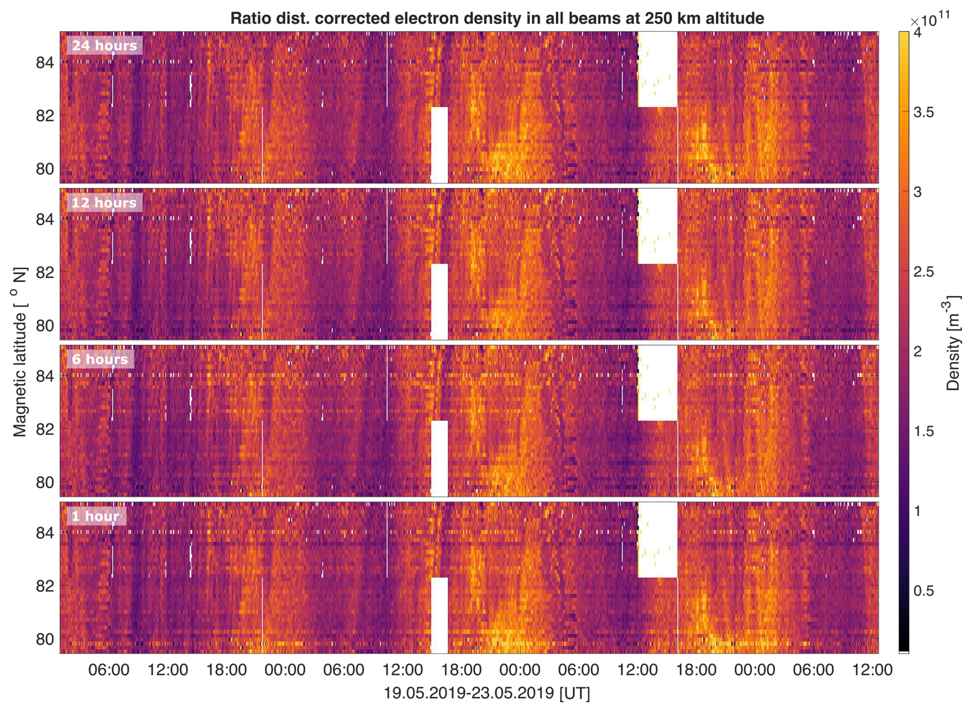
Figure 6 Corrected electron density at 250 km altitude from 38 beams during the experiment presented in example 3, Fig. 3. In each panel, a randomly chosen subset of the full dataset from the experiment was used to calculate the correction factor from the ratio distribution of the electron density ratios (Method 2). The top panel shows the result for using a 24 h subset of data, the second for 12 h, and the two bottom panels show the result for a 6 and 1 h subset of data. The subsets are chosen randomly from the 3.5 d dataset.

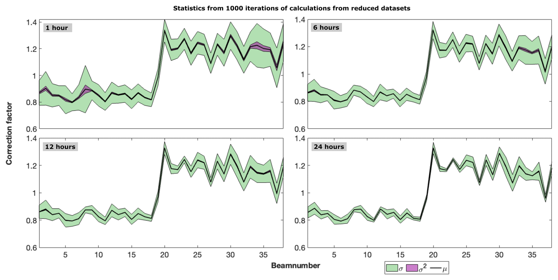
Figure 7 The standard deviation and variance of the calculated correction factors when using subsets of a larger dataset. The calculations for the correction factor are repeated 1000 times using a 1, 6, 12, and 24 h, randomly chosen subset of data. The standard deviation and variance of these iterations are indicated by the green and purple shaded areas, respectively. The black line indicates the mean of the iterations and will converge to the same values as for calculations done once using the full dataset.

The second approach used to assess the robustness of our method is by fitting a Gaussian function to the Kernel density estimate of the distribution of $N_{\mathrm{e}}^{\text{ratio}}$. The density function from the Kernel density estimate is not expected to resemble a Gaussian function as a whole, as electron density data generally contains data from transient events like polar cap patches, auroral events, or precipitation events that are not expected to be normally distributed throughout an experiment. The $N_{\mathrm{e}}^{\text{ratio}}$ corresponding to the peak probability density indicates the most common ratio for the given beam at the given altitude for the current experiment. By fitting a Gaussian function to the Kernel density estimate in close proximity to this maximum, we can calculate the width of the Gaussian. This is used as a measure of the standard deviation of the $N_{\mathrm{e}}^{\text{ratio}}$ distribution and leads us to an estimate of the uncertainty of the correction factor. Additionally, the standard error of the mean can be calculated. The mean is the centre of the Gaussian distribution, which corresponds to the $N_{\mathrm{e}}^{\text{ratio}}$ value at which the peak of the probability density occurs. This is done for the three examples presented above in Figs. 3–5. Figure 8 shows the calculated correction factors (y axis) using our method at the respective altitudes as presented in the Figures above. The purple line indicated the correction factors calculated when using the electron density from the fit of the ISR spectrum, while the red line indicated the correction factors when using the electron density calculated from the backscattered power of the radar signal. The standard deviation and standard error of the mean of the fitted Gaussian function are indicated for each beam (x axis), by the yellow and orange bars, respectively.

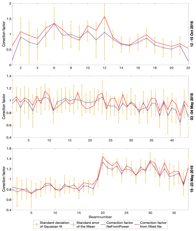
Figure 8 The standard deviation and standard error of the mean of the fitted Gaussian distribution to the ratio distributions giving the correction factors, for the three experiments presented as examples in Figs. 3–5. These are calculated at 250 and 200 km altitude at all beams respectively, corresponding to the altitudes shown in the examples. The purple line indicates the correction factors as calculated from the raw electron density, while the red line indicates the correction factors calculated from the fitted electron density.

5 Discussion

We present a method to improve the calibration of multi-beam ISR electron density data. The method calculates a correction factor, G, that is subsequently used to scale the electron density measurements. It is similar to the adjustments of the magic constant and system constant used by the EISCAT and AMISR radars, respectively (see Eq. 5). The magic constant and system constant are inferred from knowledge of the radar system and the characteristics of the antenna pattern and radar parameters used for a given experiment. In contrast, the correction factors obtained from the method described here are determined from the multi-beam electron density data itself. For this, either the electron density from the ISR spectra fit or from the backscattered power of the signal could be used. Thus, our proposed method does not attempt to replace current calibration methods but rather adds a second-level calibration correcting for variable, unpredictable, and unaccounted variations in system gain. As such, this procedure should be considered as an integral part of the data-processing chain for every multi-beam ISR.

The method is based on the established Flat field calibration method used in imaging and photography (see e.g. Burke, 1996, and references therein.). It uses a statistical approach, considering the distribution of the measurements, to estimate G. Here, the distribution of electron density ratios for each beam are found. Through a Kernel density estimate, we obtain the estimated correction factor, which is used to obtain corrected electron density measurements.

In the case of good/ideal basic (first-level) calibration, this additional calibration method scales all electron densities with a factor of G=1 in each beam. If there are unaccounted variations the method contributes to a near ideal calibration. Additionally, for the case where the electron density in one beam is accurately calibrated, e.g. with a plasma line measurement, all calibration factors should then be scaled such that the calibration factor of that beam is G=1. Lacking a beam with such accurate calibration, there will be one system-wide calibration scaling uncertainty. The calibration method presented here is also useful for future experiments and future radars like EISCAT 3D, where data volume is an issue, as it would reduce the need for a plasma line measurement in every beam.

One notable result of our method is observed in Fig. 2, where it is clear that different correction factors calculated from the raw electron density (/NeFromPower/Ne_NoTr for AMISR data) vary with range within the same beam. The received signal power in the radar should decrease by a factor of $\frac{\mathrm{1}}{R^{\mathrm{2}}}$ with range only. There should be no range dependence in the correction factor. It is unclear why this is observed.

A possible explanation could be that there is a Faraday-rotation of the signal as it propagates through the ionospheric plasma and scatters back. If the polarization of the transmitted signal is only circular in the bore-sight directions, which would be the case for a phased-array radar transmitting at peak power, off-boresight beams would have slightly elliptical polarization. For example, assuming a parallel magnetic field component of 52 000 nT, a total electron content of 10 TECu, the Faraday rotation would be approximately 72° for a 440 MHz EM wave. Radars, such as Irkutskt ISR do observe Faraday rotation effects in power for off-boresight beams (Alsatkin et al., 2020), where the transmitted polarization is elliptic, and the received polarization ends up not being matched to the transmitted polarizations

However, investigating this in full depth should be the objective of a follow-up study. If there are remaining structures in the electron densities, as shown in Figs. 3–5, from the fits of the ion-line spectrum, this procedure can be applied to those electron-densities such that those structures are reduced, regardless of the reason for such systematic structures to appear.

In Sect. 3 it was shown that there is sometimes a need to compensate for irregularities and nonphysical step-changes in the calibration of multi-beam electron density data from ISRs. Additionally, there is no way to determine which radar beam is the “correct” one without a separate, independent measurement. The presented examples show that our method improves calibration and data usability. This is especially valuable for research where quantitative, inter-beam comparisons of electron density changes are of interest, e.g., studies of plasma patches, irregularities, and turbulence. Although there is a general need for accurate independent measurements for optimal calibration, we argue that by applying this method, the electron density measurements in all pointing directions within one experiment become inter-calibrated. An effort was made to analyze the quality and robustness of the method in Sect. 4.

One challenge of this method is considered in Fig. 7. Although it can efficiently be applied to any multi-beam ISR experiment, it is somewhat sensitive to the length of the dataset. That is, to acquire a good Kernel density estimate of the ratio distribution, an adequate number of measurements is required. Figure 7 illustrates this as it is clear that the results of the correction become progressively worse when reducing the number of measurements. This means that there is a minimum number of measurements needed to acquire a reasonable result. The required number of measurements changes depending on the experiment and data resolution. However, the result illustrated in Fig. 7 indicates that a 12 h experiment duration produces a noticeable improvement in the RISR experiment used as an example.

6 Conclusions

Calibration of ISR is a complex and difficult task, especially when independent measurements of the electron density are only available in one pointing direction or not at all. We have proposed a method for the correction of electron density measurements from multi-point ISRs. This method is intended to add to the current efforts that are made for the calibration of multi-point radars and can increase data usability and quality by considering variable, unaccounted and, unpredictable variations in system gain. It is based on the well-established Flatfield correction method in imaging and photography. We exploit the similarity between independent measurements in separate pixels in one image sensor and multi-beam radar measurements. The correction factors are estimated based on a Kernel density estimate of the distribution of $N_{\mathrm{e}}^{\text{ratio}}$ calculated from all measurements of an experiment. This is subsequently used to estimate the correction factor. The method is robust and efficient for the examples presented here. It is sensitive to the length of the experiments when these are well below 12 h. The errors and robustness of the method were estimated through two different approaches. Accurate independent measurements are needed to determine absolute values of electron density and an optimal calibration. However, we argue that by applying the presented method, the electron density measurements in all pointing directions within one experiment become intercalibrated. Thus, this second-level calibration is especially valuable for studies of plasma patches, irregularities, turbulence, and other research where inter-beam changes of electron density are of interest.

The presented method is strictly based on the observed electron density data and requires no additional input. It is efficient and its application on existing and future data is straightforward. Additionally, it requires minimal user input and is not expected to increase the demand for computing power. Thus, we suggest that it be implemented and applied as a second-level calibration in future calibration schemes of multi-point radars where any calibration is required. This will improve the calibration and data accuracy of phased array incoherent scatter radar measurements and thus overall data usability and quality.